Circuit Theory 2 · AC Kirchhoff laws, nodal analysis and mesh analysis
#04 Use impedance and admittance to write series-loop, parallel-node and coupled-mesh equations
Keep Kirchhoff's laws, replace ideal elements by impedances, and derive the series, node and two-mesh equations with explicit sign conventions.
Question
Apply Kirchhoff's voltage law (KVL) and current law (KCL) to ideal lumped linear time-invariant R, L and C networks in sinusoidal steady state at one common positive angular frequency ω, using e^(jωt). R, R1, R3, L and C are positive constants. Uppercase V and I are phasors, not instantaneous waveforms; choose one common peak or RMS convention. For the series R–L loop, take clockwise current and Vs as the source upper-terminal voltage minus its lower-terminal voltage; use passive voltage drops along the current. For the parallel R–C example, define the bottom rail as the zero-voltage reference, V as top minus bottom, source current into the top node and resistor/capacitor branch currents downward. Derive the total admittance in siemens, then divide only by a nonzero coefficient. For the two-mesh network, define both currents clockwise and Vs positive at the source upper terminal. R1 is exclusive to loop 1, R3 is shared, and L with C lie in the outer branch of loop 2. Explain the downward shared-branch current I1−I2 and derive both coupled equations. The original mesh drawing uses counterclockwise arrows and leaves source polarity unmarked; the notebook states its chosen references explicitly and uses a different same-video reference card, not a newly corrected circuit. Separate equations are required for different frequencies in a linear superposition problem; do not add their phasors as if they had one frequency. Convert to time domain only after solving, keeping cosine/sine and peak/RMS conventions consistent. Original audio/video are unchanged; legacy raster readability and source diagram issues remain manual publication-QA items.
Written solution and narration transcript(shows the full solution)
Below are all the lines written in the notebook together with the full narration transcript.
1. Keep Kirchhoff laws at a common sinusoidal frequency
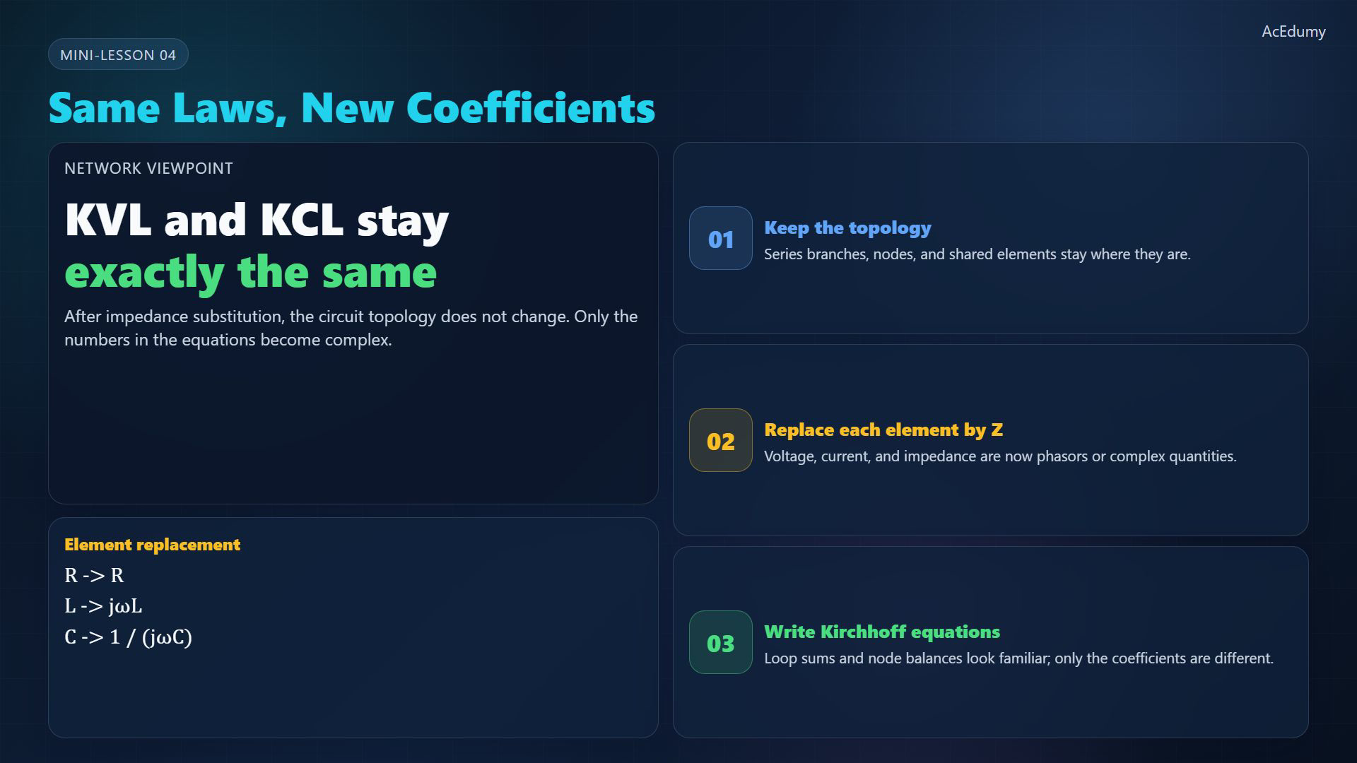
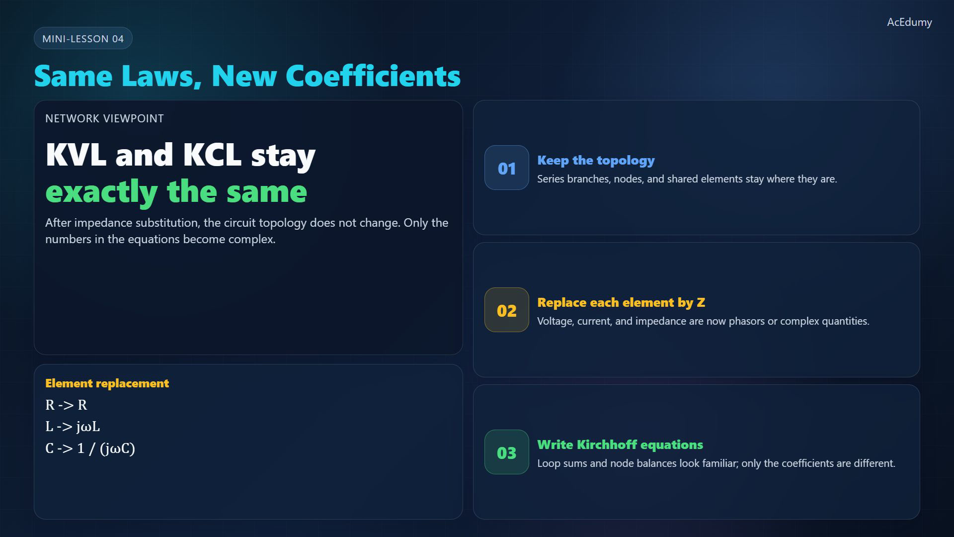
Reference from the original video. Readable notebook equations state the model, current directions and voltage references; legacy cards are not newly corrected circuit diagrams. Use ideal, lumped, linear time-invariant elements in sinusoidal steady state at one common positive frequency.Replacing an element by its impedance keeps the same electrical connections.Kirchhoff's voltage law (KVL) sums signed loop voltages; Kirchhoff's current law (KCL) balances signed node currents.With the positive-frequency convention, L and C introduce complex coefficients. R remains real; phasor voltage and current use one common peak or root-mean-square (RMS) convention.Narration transcript
In the last lesson, we turned R, L, and C into impedances. Once that replacement is done, the network laws do not change shape. Kirchhoff's voltage law is still a loop sum, and Kirchhoff's current law is still a node balance. The only real difference is that the coefficients are now complex.
2. Write the series R–L loop equation
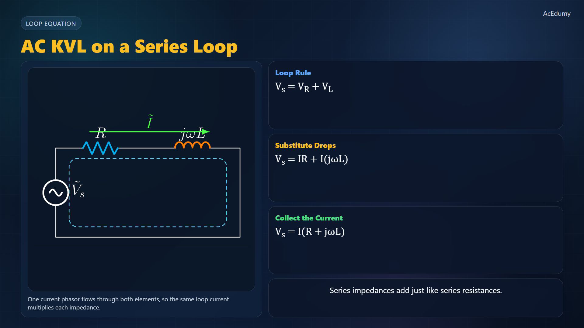
Reference from the original video. Readable notebook equations state the model, current directions and voltage references; legacy cards are not newly corrected circuit diagrams. For the series R–L loop, choose clockwise current; the source voltage is top minus bottom.Take passive voltage drops along the current:Substitute the two drops and factor the same current:The series impedance is the sum, in ohms:Narration transcript
Start with A C K V L. In a series R L loop, the source phasor equals the sum of the element drops. So V sub s equals I R plus I j omega L, or I times the quantity R plus j omega L. Same loop rule, same topology, new impedance labels.
3. Balance currents in the parallel R–C circuit

Reference from the original video. Readable notebook equations state the model, current directions and voltage references; legacy cards are not newly corrected circuit diagrams. At the parallel R–C node, define V as the top-node voltage relative to the bottom rail, chosen as zero.Source current enters the top node; both branch currents leave downward:Both branches have the same top-to-bottom voltage:For positive frequency, capacitor admittance is jωC, so:Factor the common node voltage without changing the current directions:Narration transcript
Now A C K C L. At a node fed by a current source, incoming current equals outgoing branch currents. If one branch is a resistor and the other is a capacitor, then I sub s equals V over R plus V over Z sub C. Since Z sub C equals one over j omega C, this becomes I sub s equals V over R plus j omega C times V. Same node logic, new complex coefficients.
4. Solve the unknown node voltage
Reference from the original video. Readable notebook equations state the model, current directions and voltage references; legacy cards are not newly corrected circuit diagrams. Nodal analysis uses the same parallel R–C circuit and bottom-rail reference.Admittances add in parallel; every term is measured in siemens:Divide by the complete nonzero admittance, not by only its first term:Check by substitution in the original node equation:For positive finite R, the admittance has a positive real part and cannot be zero. General circuits still require checking whether the equations have a unique solution.Narration transcript
This is why node analysis still works. If the node voltage V is the unknown, collect the admittances connected to that node. For this example, V equals I sub s over the quantity one over R plus j omega C. The workflow is still isolate the unknown and solve. The only change is that the coefficient is complex instead of purely real.
5. Couple the two mesh-current equations
Reference from the original video. Readable notebook equations state the model, current directions and voltage references; legacy cards are not newly corrected circuit diagrams. Choose both mesh currents clockwise and the source positive at its upper terminal. These are explicit notebook references; the old diagram uses different arrows and leaves polarity unmarked.Loop 1 contains R1 and the shared resistor R3; its downward shared current is I1−I2:Loop 2 has R3, L and C, with no independent source in that loop:Solve the two equations together using complex arithmetic. A shared-branch current is a difference of mesh currents, not either mesh current alone.Narration transcript
Mesh analysis also survives intact. Define mesh currents I one and I two exactly as before, then write A C K V L around each loop using impedances. The shared resistor couples the two equations, so the result becomes a small complex linear system. You solve it the same way you would in D C, just with complex arithmetic.
6. Apply the three-step impedance-domain recipe
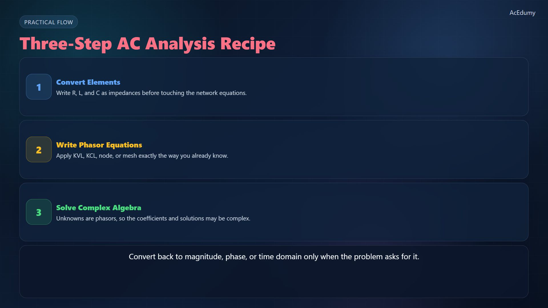
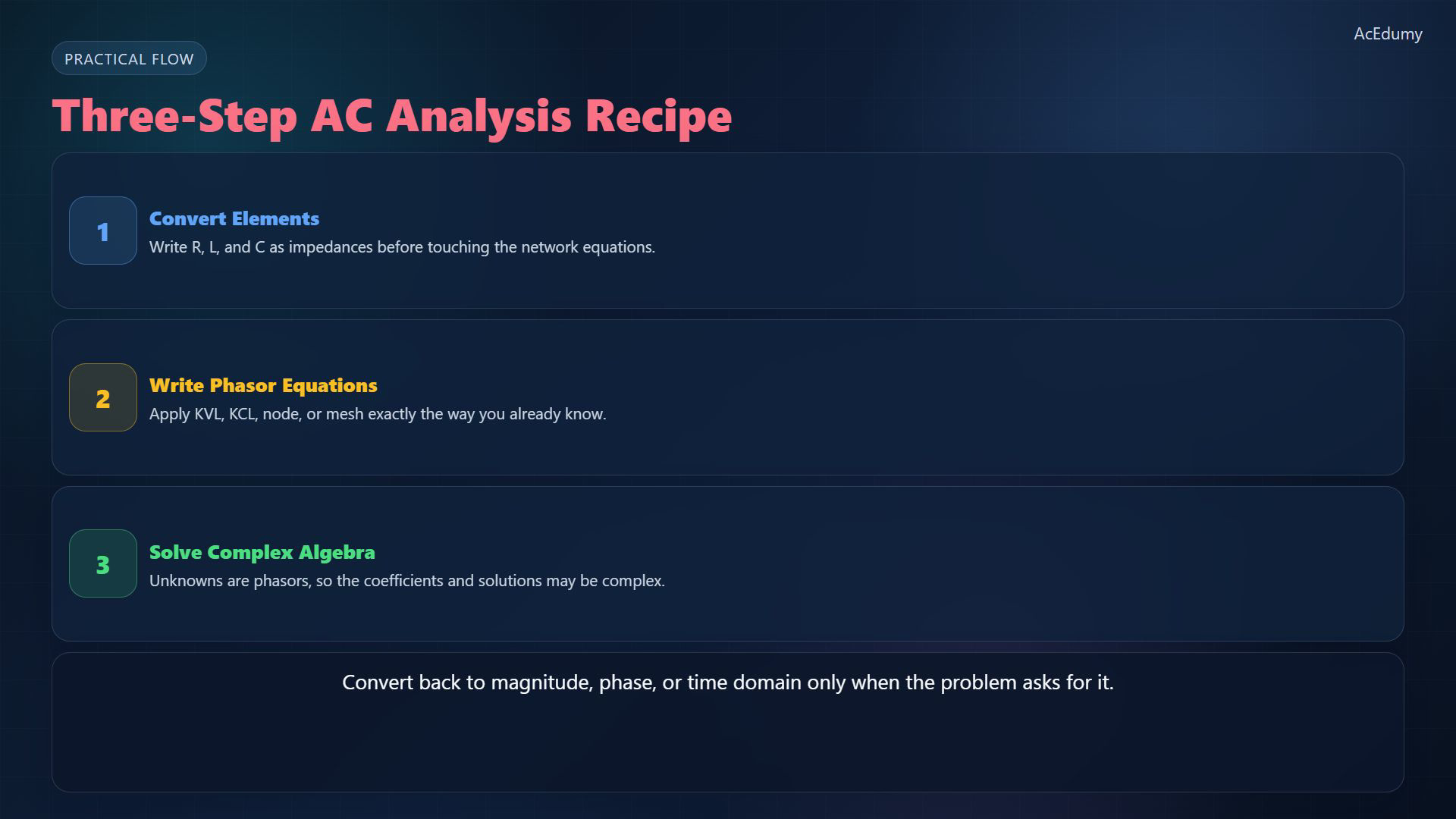
Reference from the original video. Readable notebook equations state the model, current directions and voltage references; legacy cards are not newly corrected circuit diagrams. Use a three-step workflow at the chosen sinusoidal frequency.First replace ideal R, L and C by their impedances. The capacitor term keeps its whole denominator:Second write signed KVL, KCL, nodal or mesh equations, keeping all voltage and current references consistent.Third solve for the unknown phasors. Different source frequencies require separate linear problems before combining time-domain responses.Only then convert to magnitude and phase or to time domain, if needed. Preserve the chosen cosine/sine and peak/RMS convention.Narration transcript
In practice, the recipe is short. First, replace R, L, and C with impedances. Second, write K V L, K C L, node, or mesh equations with phasors. Third, solve the complex equations for the unknown phasors. After that, convert back to magnitude and phase, or to the time domain, only if the problem asks for it.
7. Connect node and mesh analysis to equivalent sources

Reference from the original video. Readable notebook equations state the model, current directions and voltage references; legacy cards are not newly corrected circuit diagrams. Alternating-current (AC) nodal and mesh analysis use the existing Kirchhoff laws within the stated lumped-circuit model.Impedance substitution changes element coefficients, not circuit connections or the requirement for consistent signs.Next: AC source transformations, Thevenin equivalents and Norton equivalents.Narration transcript
So A C node and mesh analysis are not new laws. They are the same Kirchhoff laws in the impedance domain. In the next lesson, we will use this viewpoint for A C source transforms, Thevenin equivalents, and Norton equivalents.
Source video: Circuit Theory-2 #04 AC KVL, KCL, Node, and Mesh (3:07)