Circuit Theory 2 · Active band-pass, band-reject and Butterworth filters

#25 Complex block composition, overall band edges, relative bandwidth and Butterworth scope

Distinguish overall band edges from individual stage corners and combine complex filter responses with explicit gain, phase and practical limits.

Question

Reviewed same-video reference about active middle-band filter parameters, design workflow or practical checks. — Reference from the same original video. Seven roles use reviewed alternative cards; the retained notch plot is schematic, not a quantitative transfer curve. Exact formulas and conditions appear in the notebook.

Study ideal real LTI stable active filter blocks with positive constant components, appropriate negative feedback and initially relaxed energy storage. Input and output are node voltages relative to a common reference. Block diagrams are not complete op-amp schematics. Buffering reduces stage loading; it is neither galvanic isolation nor infinite bandwidth or unlimited output current. Track signed gains and phase: cascade multiplies complex transfer functions, a summer adds complex weighted responses, not magnitudes. For an illustrative mathematical example with positive unity passband gains, H_HP(s)=s/(s+a), H_LP(s)=b/(s+b), a,b>0. Their product H_BP=b*s/((s+a)(s+b)) has stable real poles−a,−b, a zero at zero and peak at ω0=sqrt(ab). Peak magnitude b/(a+b), not necessarily1. Relative half-magnitude-squared edges satisfy |ab−ω²|=(a+b)ω: ω1=(sqrt((a+b)²+4ab)−(a+b))/2, ω2=(sqrt((a+b)²+4ab)+(a+b))/2. Thus Δω=a+b,ω1ω2=ab,Q=sqrt(ab)/(a+b)<=1/2. The stage corners a,b are not these overall edges; even a=b gives finite width2a, peak1/2 and edges(sqrt2∓1)a, not zero width. Choose a<b for a broad overlapping useful region; selectivity cannot be made arbitrarily high with two first-order real-pole sections. Two actual inverting stages may have positive product; any added inverting gain must still be included. Cascade order is mathematically commutative under the ideal no-interaction assumption, though practical loading and headroom can differ. The source order/overlap shorthand does not establish ideal brick-wall rejection. For a two-path sum, drive both paths from the input and connect them to separate summer inputs, never short amplifier outputs. Include signed weights k1,k2 and all phase shifts. Equal-corner positive unity LP+HP=a/(s+a)+s/(s+a)=1; it is an identity, not a notch. For an explicit separated-path example use LP=a/(s+a) and HP=s/(s+b) with0<a<b. Their sum=(s²+2as+ab)/(s²+(a+b)s+ab) tends to1 at both extremes, has center sqrt(ab) and finite minimum2a/(a+b), never an exact zero for positive a. Two relative half-magnitude-squared edges in this example require(a+b)²−8a²>0; an arbitrarily shallow dip may have no such edges. A target standard second-order notch H_N=(s²+ω0²)/(s²+(ω0/Q)s+ω0²),Q>0, has an exact imaginary-axis zero and relative reject widthω0/Q. This is a target model, not a derivation from the source's unspecified LP/HP blocks. With the earlier cascade, 1−((a+b)/b)H_BP creates this real-pole notch mathematically, emphasizing weighted complex cancellation rather than arbitrary addition. A sharper Q needs appropriate second-order sections. Phase is undefined at an exact zero. The geometric center and Q/width identities refer to these specified standard models and measured relative edges, not every arbitrary high-order response. Minus3dB is a rounded label for−3.0103dB at magnitude1/sqrt2 relative to peak/passband; no unconditional power-transfer claim for arbitrary port impedances. ω is angular frequency, f=ω/(2π); Q dimensionless. Higher Q means narrower relative width at fixed center. Ideal Butterworth low-pass prototype magnitude=1/sqrt(1+(ω/ωc)^(2N)), positive integerN. Squared magnitude's first2N−1 derivatives vanish atω=0; monotonic/ripple-free is not perfectly flat over the entire passband and says nothing about linear phase. At cutoff relative magnitude1/sqrt2. Exact logarithmic slope−20N*x^(2N)/(1+x^(2N)),x=ω/ωc, gives−10N dB/decade at cutoff and tends to−20N far above it. The spoken20/40 values describe these remote low-pass asymptotes, not constant slopes immediately past the edge, nor−40 on both sides of every second-order band-pass. For the illustrative band-pass the remote slopes are+20 and−20; a notch returns to its high-frequency passband. Proper low-pass-to-band transformations are needed for Butterworth band responses; a prototype orderN typically maps to total band-pass order2N, not a blanket20 times total order on each side. Assess op-amp loop/noise gain, stability, bandwidth, slew, swing, load, noise and component sensitivity; no device purchase or circuit publication approved here. All133 audio-source/357TSX/434graph lines and EN metadata read. Original final254.784s and all11MP3+timings13sourceSHA match. Cached-large ASR .9167–1 recognizes every passage and critical20/40/omega/Q statement;51 original aligned cues reviewed,29–59ms MP3/final offsets and correlations .96226–.98601. No numeric/sign speech error demonstrated; source shorthand is explicitly scoped, not silently repaired or claimed full teaching approval. All11 final frames reviewed. Seven roles use same-final alternatives: middle-band-goal→bridge,bandpass-cascade→design-workflow,bandpass-equation→design-workflow,bandreject-path→practical-limits,butterworth→design-workflow,order-slope→practical-limits,summary→bridge. Middle-band curves use empirical shapes and preset edge markers not computed from the complete transfer functions. Band-pass parameter plot has a misleading numeric0dB tick and uncomputed edge locations. Cascade output label overlaps its arrow and wording blurs stage/overall edges. Sum input branching is visually ambiguous near its label and its unqualified missing-middle caption overflows; no two-output short is inferred or reproduced. Butterworth−3dB tick does not match linear-magnitude geometry and grey ripple curve is illustrative, not a specified Chebyshev response. Order graph labels−40/−80 but uses linear magnitude and its fourth-order legend spills below panel. Wrap's LP-plus-HP rule lacks conditions. Retained band-reject parameter frame is a schematic Gaussian dip with arbitrary markers, not an analytic quantitative response or guaranteed notch zero; readable formulas refer only to the explicit standard model. Retained workflow has invisible colored-square step numbers and fifth-card text near its border, but headings/body remain readable; practical card readable. Original say,MP3,video and51cue boundaries unchanged; no alignment overrides,prompts,threshold changes,newTTS,video render,paid service or publication. Four unique original reference frames across eleven roles. Unpublished technical draft; complete human listening, motion QA and teaching/publication approval remain outstanding.

Written solution and narration transcript(shows the full solution)

Below are all the lines written in the notebook together with the full narration transcript.

1. Combine the previous active filter blocks
Reference from the same original video. Seven roles use reviewed alternative cards; the retained notch plot is schematic, not a quantitative transfer curve. Exact formulas and conditions appear in the notebook.
Use the previous active low-pass and high-pass sections as linear filter blocks.
Each block has a complex transfer function, not just a magnitude shape.
Choose block connections, gain signs and frequency ranges together.
Suitable cascade or weighted summation can keep or attenuate a middle band; arbitrary ordering alone does not guarantee a notch.
Narration transcript
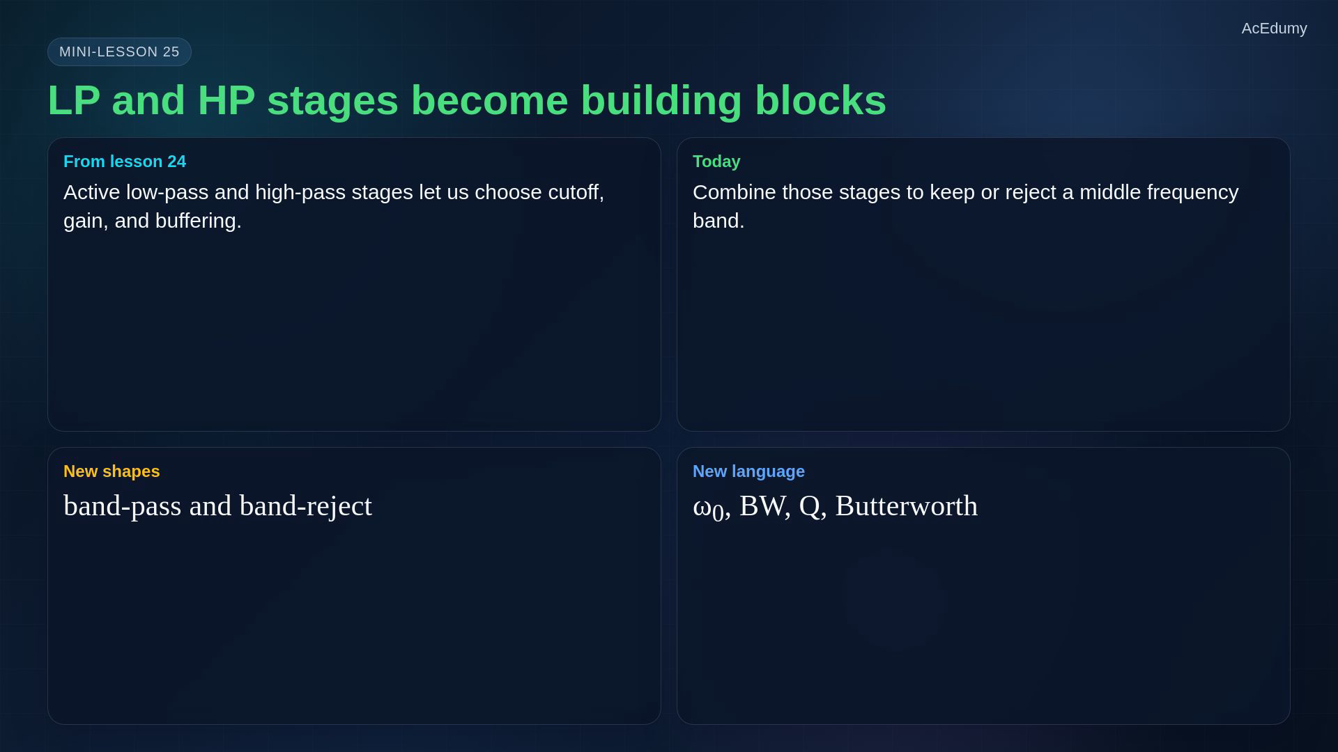
In the last lesson we used op-amps to make active low-pass and high-pass filters. Those two blocks are more than separate examples. They are building blocks. If we place them in the right order, we can keep only a middle band, reject a middle band, and control how smooth or sharp the transition looks.
2. Define measured band edges
Reference from the same original video. Seven roles use reviewed alternative cards; the retained notch plot is schematic, not a quantitative transfer curve. Exact formulas and conditions appear in the notebook.
Define two edges of the complete response, with a stated magnitude reference.
Here the lower and upper overall edges are ordered:
$\displaystyle \omega _{1}<\omega _{2}$
A band-pass retains the middle region relative to its own peak.
Outside the chosen band it attenuates; a physical finite-order filter does not erase every outside frequency.
A band-reject attenuates the middle while retaining both sides; removal is not zero gain over an entire interval.
Narration transcript
A middle-band filter has two important edge frequencies. The lower edge starts the useful band, and the upper edge ends it. Between them, the band-pass filter keeps the signal. Outside them, it attenuates. The band-reject filter does the opposite: it keeps low and high frequencies but removes the middle region.
3. Cascade high-pass and low-pass stages
Reference from the same original video. Seven roles use reviewed alternative cards; the retained notch plot is schematic, not a quantitative transfer curve. Exact formulas and conditions appear in the notebook.
Ideal unloaded cascade multiplies the complex stage responses:
$\displaystyle H_{\mathrm{BP}}\left(s\right)=H_{\mathrm{HP}}\left(s\right) H_{\mathrm{LP}}\left(s\right)$
For an illustrative positive unity-passband high-pass stage with positive corner a:
$\displaystyle H_{\mathrm{HP}}\left(s\right)=\frac{s}{s+a}$
Follow it with an illustrative positive unity-passband low-pass stage with corner b:
$\displaystyle H_{\mathrm{LP}}\left(s\right)=\frac{b}{s+b}$
Suitable buffering reduces interaction; it does not remove bandwidth, stability or source/load limits.
Overall edges must be calculated from the product, not copied from a and b:
$\displaystyle H_{\mathrm{BP}}\left(s\right)=\frac{b s}{\left(s+a\right)\left(s+b\right)}$
Narration transcript
The simplest active band-pass idea is a cascade. First use a high-pass stage to remove low frequencies. Then use a low-pass stage to remove high frequencies. Because the stages are active and buffered, the second stage does not strongly disturb the first stage. The useful band is the overlap between them.
4. Distinguish stage corners from overall edges
Reference from the same original video. Seven roles use reviewed alternative cards; the retained notch plot is schematic, not a quantitative transfer curve. Exact formulas and conditions appear in the notebook.
Use the overall half-magnitude-squared edges relative to the band-pass peak, not the individual stage corners.
Angular bandwidth is the difference of those overall edges:
$\displaystyle \Delta \omega =\omega _{2}-\omega _{1}$
For the specified second-order band-pass model the center is geometric:
$\displaystyle \omega _{0}=\sqrt{\omega _{1} \omega _{2}}$
Quality factor is dimensionless and describes relative width:
$\displaystyle Q=\frac{\omega _{0}}{\Delta \omega }$
Narration transcript
For a band-pass response, we usually name the lower edge omega one and the upper edge omega two. The bandwidth is omega two minus omega one. The center frequency is the geometric mean: omega zero equals the square root of omega one times omega two. Then Q equals center frequency divided by bandwidth.
5. Sum properly separated complex paths
Reference from the same original video. Seven roles use reviewed alternative cards; the retained notch plot is schematic, not a quantitative transfer curve. Exact formulas and conditions appear in the notebook.
Split the input into two independent paths and combine their outputs through a summer, never by shorting amplifier outputs.
The low-pass path retains low frequencies; its corner must be chosen for the intended rejected band.
The high-pass path retains high frequencies; include signed summer weights and phase:
$\displaystyle H_{\mathrm{BR}}\left(s\right)=k_{1} H_{\mathrm{LP}}\left(s\right)+k_{2} H_{\mathrm{HP}}\left(s\right)$
Important qualification to the source shorthand; equal-corner unity complementary paths give no rejection at all:
$\displaystyle \frac{a}{s+a}+\frac{s}{s+a}=1$
Narration transcript
A band-reject filter can be understood as two paths added together. One path is low-pass, keeping the low-frequency part. The other path is high-pass, keeping the high-frequency part. When the middle band is missing from both paths, the output has a notch or rejected band.
6. Distinguish a rejected band from an exact zero
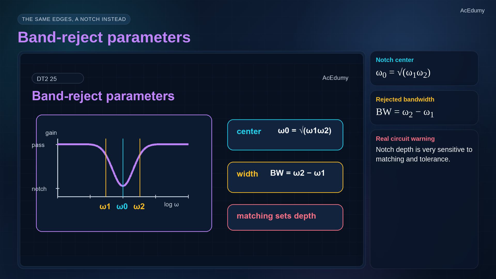
Reference from the same original video. Seven roles use reviewed alternative cards; the retained notch plot is schematic, not a quantitative transfer curve. Exact formulas and conditions appear in the notebook.
Define reject edges relative to the actual passband, not relative to the notch floor.
The lower and upper reject boundaries belong to the complete response.
A standard second-order target notch, not an automatic result of any two-path sum, is:
$\displaystyle H_{N}\left(s\right)=\frac{s^{2}+\omega _{0}^{2}}{s^{2}+\left(\frac{\omega _{0}}{Q}\right)s+\omega _{0}^{2}}$
A deep zero needs the intended complex cancellation; component, gain and phase mismatch can fill it.
Narration transcript
The same edge-frequency language still works for band-reject filters. Omega one and omega two mark the two sides of the rejected band. The center frequency sits between them, and the bandwidth tells us how wide the notch is. In a real circuit, notch depth depends strongly on matching and component tolerance.
7. State Butterworth flatness precisely
Reference from the same original video. Seven roles use reviewed alternative cards; the retained notch plot is schematic, not a quantitative transfer curve. Exact formulas and conditions appear in the notebook.
Butterworth names a response family.
For an ideal normalized low-pass prototype of positive integer order N:
$\displaystyle |H\left(j\omega \right)|=\frac{1}{\sqrt{1+\left(\frac{\omega }{\omega _{c}}\right)^{2N}}}$
Maximally flat at zero frequency means no ripple, not constant gain throughout passband; at cutoff:
$\displaystyle |H\left(j\omega _{c}\right)|=\frac{1}{\sqrt{2}}$
Flatness trades against other design requirements; a different response family may transition faster for a specified order and ripple allowance.
Narration transcript
Now add one design word: Butterworth. A Butterworth response is chosen for a maximally flat pass band. That means no ripple in the pass band, and a smooth roll-off after the edge. It is not the sharpest possible transition, but it is clean, predictable, and very common.
8. Use asymptotic order and slope within scope
Reference from the same original video. Seven roles use reviewed alternative cards; the retained notch plot is schematic, not a quantitative transfer curve. Exact formulas and conditions appear in the notebook.
The next slope rule concerns the far high-frequency side of an all-pole low-pass, not every side of a band-pass or notch.
A first-order all-pole low-pass approaches twenty decibels of attenuation per tenfold frequency increase, well beyond cutoff.
A second-order all-pole low-pass approaches forty decibels per tenfold increase; its normalized asymptote is:
$\displaystyle G_{\mathrm{dB}}\left(\omega \right)\approx -40 \log _{10}\left(\frac{\omega }{\omega _{c}}\right)$
Higher low-pass order steepens the asymptote, but requires suitable sections; a second-order band-pass has different slopes on its two sides.
Narration transcript
Filter order controls how fast the curve falls after the edge. A first-order section rolls off at about twenty decibels per decade. A second-order section gives about forty decibels per decade. Higher order filters are sharper, but they need more stages and more careful component choices.
9. Specify edges, family and realizable stages
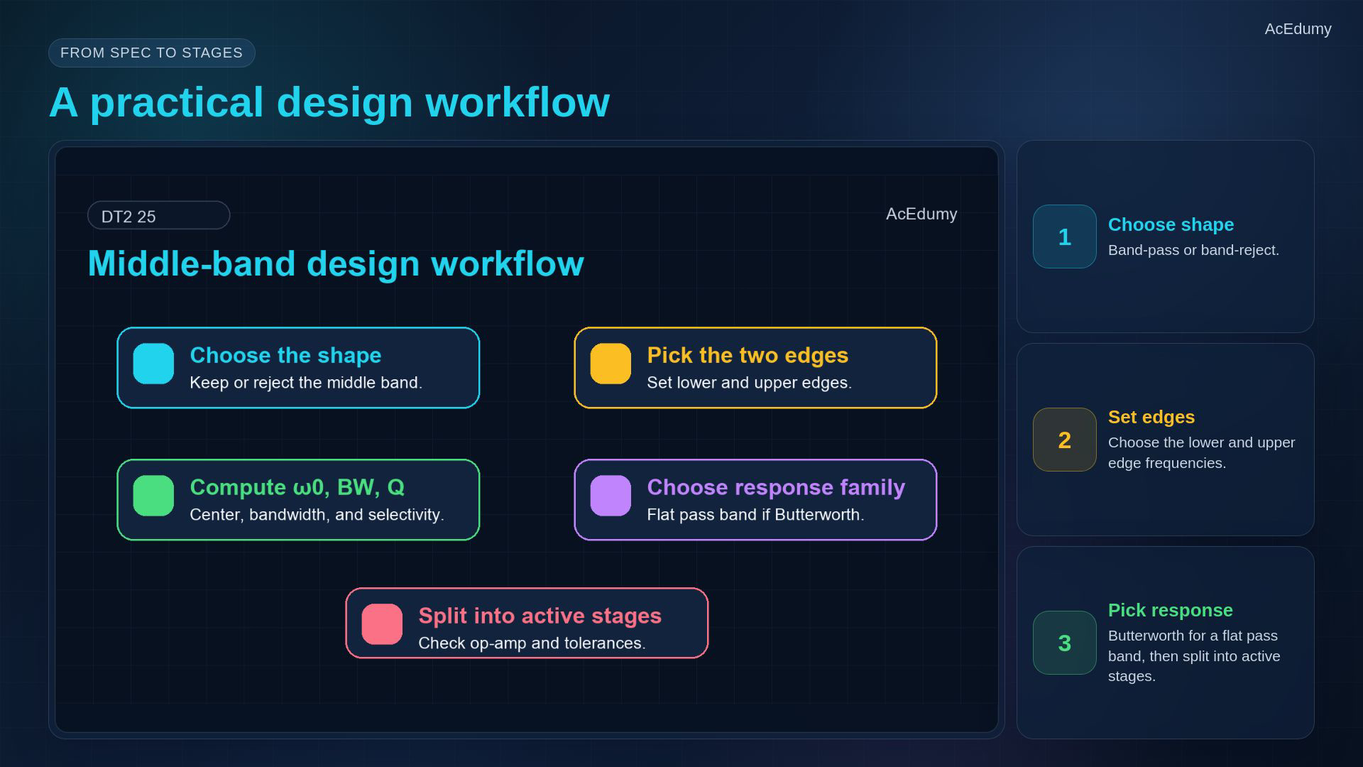
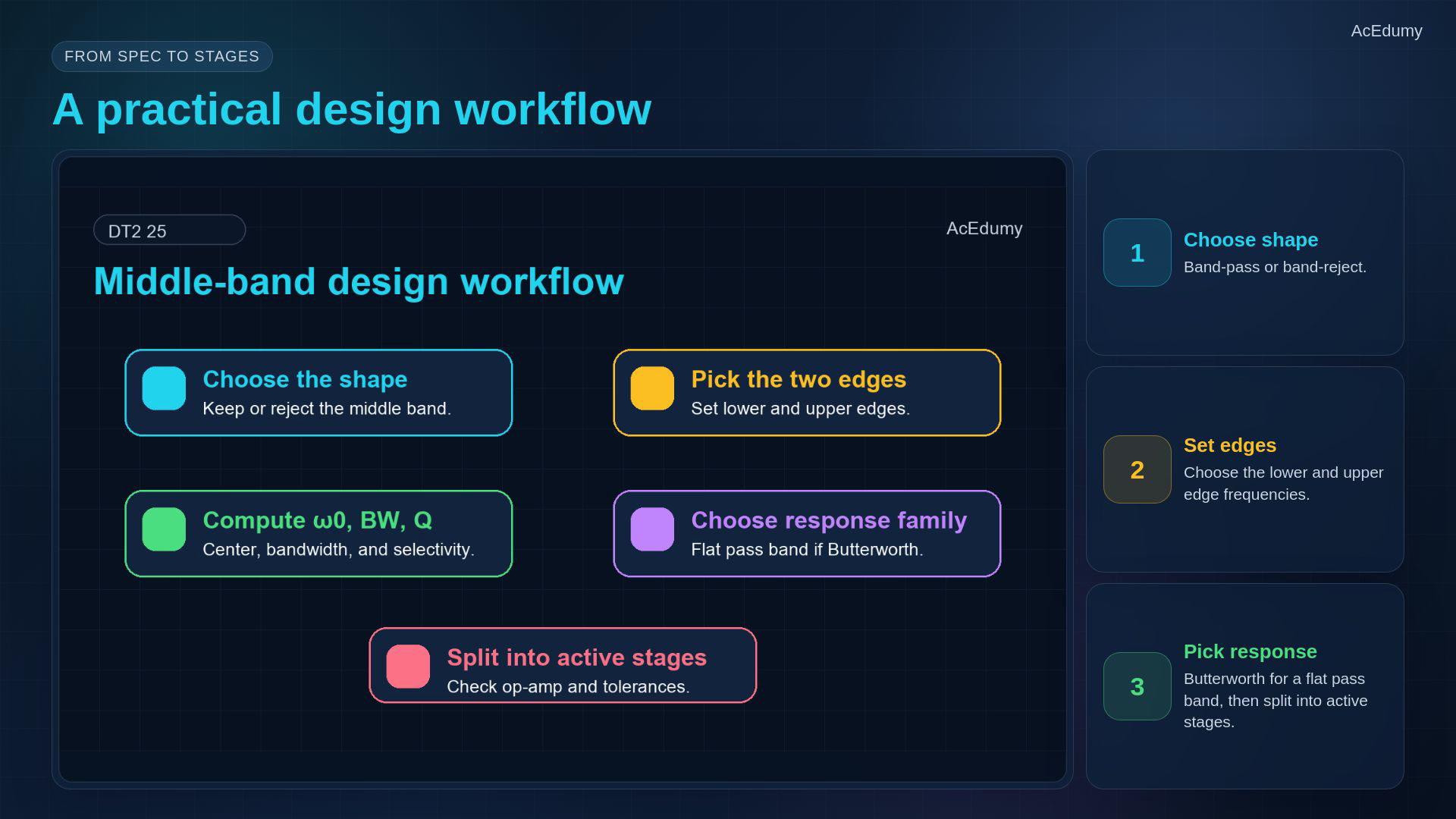
Reference from the same original video. Seven roles use reviewed alternative cards; the retained notch plot is schematic, not a quantitative transfer curve. Exact formulas and conditions appear in the notebook.
Start with the required complete response.
Specify whether the middle region must pass or be attenuated, together with gain and attenuation limits.
Choose overall lower and upper edges and their reference level.
Calculate center, width and quality factor consistently; convert angular width to hertz using:
$\displaystyle \Delta f=\frac{\Delta \omega }{2\pi }$
Choose a response family; a Butterworth band-pass or band-reject needs the appropriate frequency transformation of the low-pass prototype.
Choose realizable sections; a simple cascade of two first-order blocks cannot supply arbitrary selectivity:
$\displaystyle Q=\frac{\sqrt{a b}}{a+b}\le \frac{1}{2}$
Narration transcript
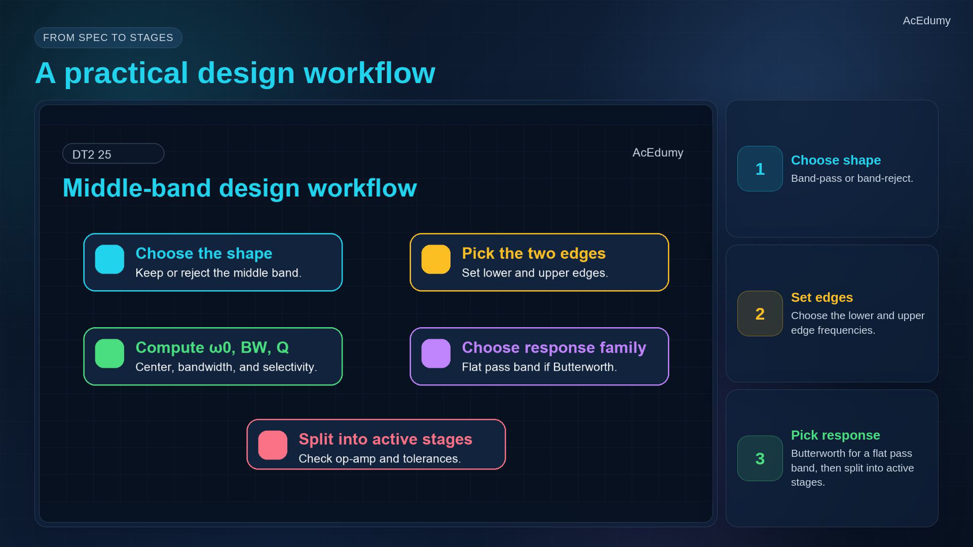
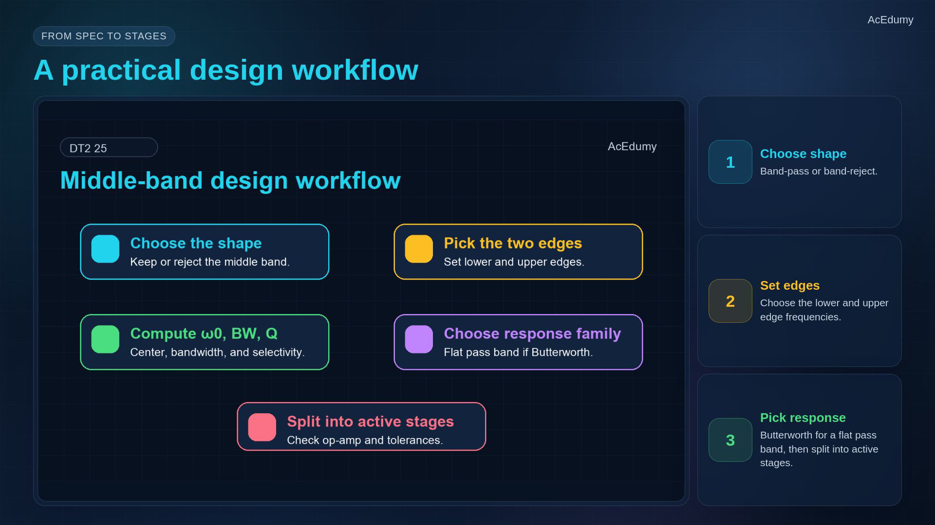
A practical workflow is this. Choose the shape: band-pass or band-reject. Choose the two edge frequencies. Compute center frequency, bandwidth, and Q. Then choose the response family, such as Butterworth for flatness. Finally, split the design into active stages that your op-amp can actually support.
10. Check nonideal gain, loading and tolerance
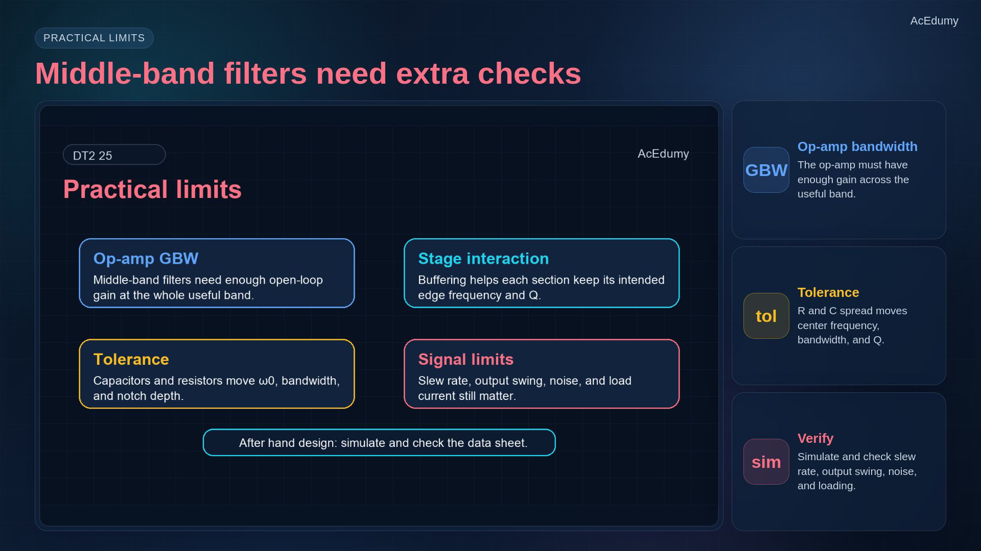
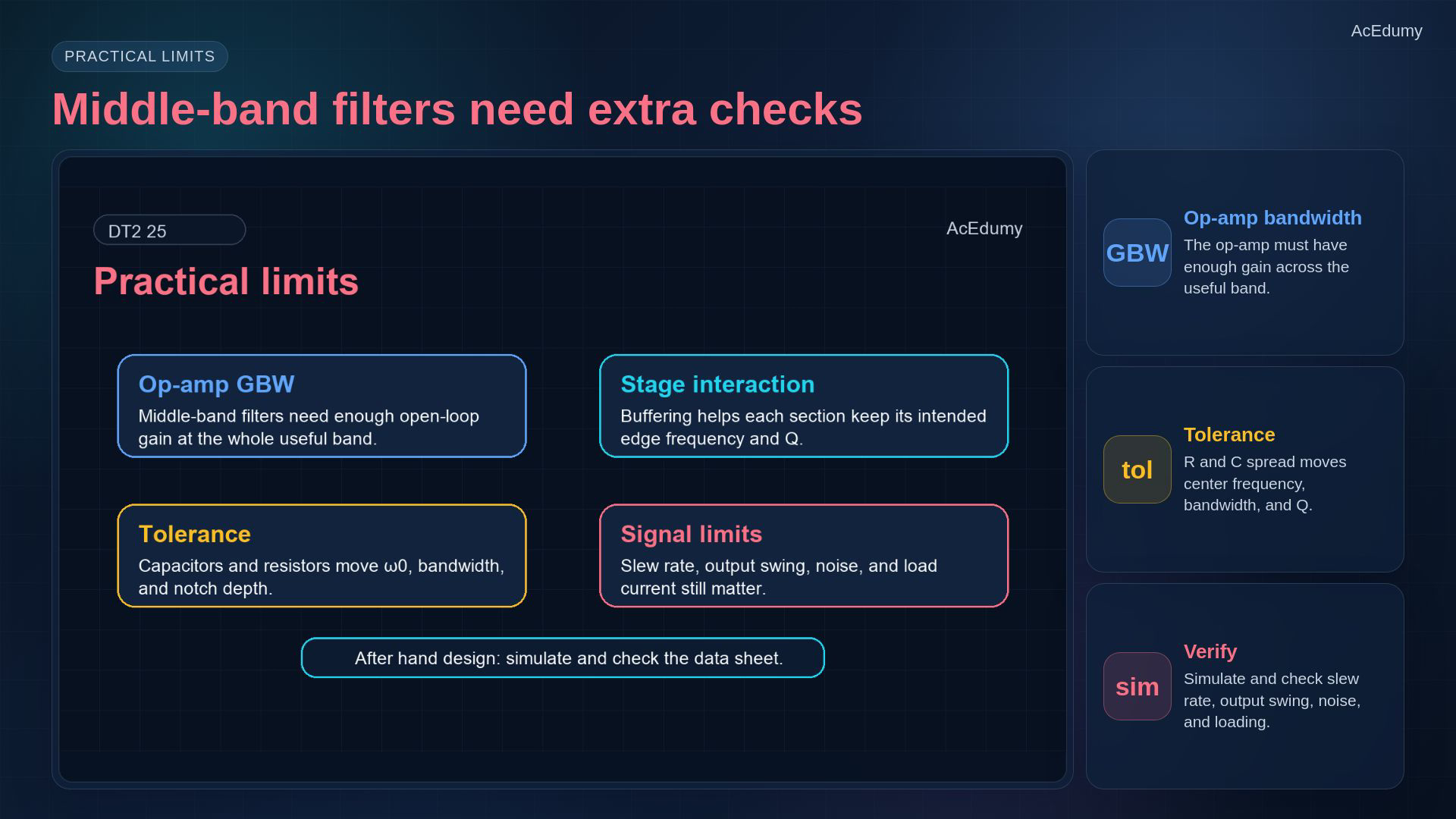
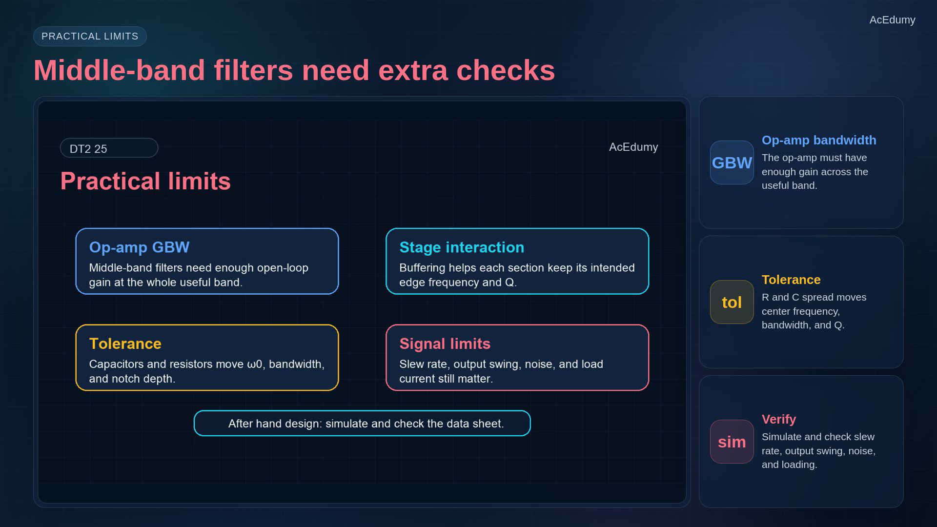
Reference from the same original video. Seven roles use reviewed alternative cards; the retained notch plot is schematic, not a quantitative transfer curve. Exact formulas and conditions appear in the notebook.
Check the chosen topology and required selectivity against real circuit limits.
Check loop gain, noise gain, usable bandwidth and stability throughout the operating band.
Buffering reduces loading between stages; it is not galvanic isolation or unlimited drive.
Capacitor tolerance can shift the center, width and other response features.
Resistor tolerance or matching can also alter center, quality factor and cancellation depth; these effects are topology-dependent.
After the ideal calculation, verify simulation and device limits, including slew rate, swing, noise and load.
Narration transcript
Middle-band active filters are sensitive to real-world limits. The op-amp needs enough gain-bandwidth. The stages need suitable buffering. Capacitor tolerance can move the center frequency. Resistor matching can change Q or notch depth. So the final circuit should be checked with simulation and with the op-amp data sheet.
11. Summarize middle-band filter design
Reference from the same original video. Seven roles use reviewed alternative cards; the retained notch plot is schematic, not a quantitative transfer curve. Exact formulas and conditions appear in the notebook.
Summary: composition and operating assumptions determine the actual band response.
Suitable cascades or weighted paths can form band-pass or band-reject behavior; adding arbitrary low-pass and high-pass paths is insufficient.
Use overall edges, geometric center where applicable, and consistent bandwidth units:
$\displaystyle \omega _{0}=\sqrt{\omega _{1} \omega _{2}}, Q=\frac{\omega _{0}}{\omega _{2}-\omega _{1}}$
Butterworth is maximally flat in the stated sense; it does not mean perfectly constant amplitude or linear phase.
Higher-order sections must realize the required poles, zeros and practical operating limits.
Narration transcript
Summary. Active low-pass and high-pass stages can be combined into band-pass and band-reject behavior. The key parameters are the two edge frequencies, center frequency, bandwidth, and Q. Butterworth is the smooth, maximally flat option. Next, we can turn this intuition into higher-order active-filter sections.