Circuit Theory 2 · Active filter design practice: specifications to stages

#26 Response specifications, pole sections, gain/noise tradeoffs, scaling and verification

Turn a filter specification into suitable sections, with explicit frequency conventions, gain/noise tradeoffs, component scaling and verification.

Question

Reviewed same-video reference for active-filter specification, sectioning, scaling or verification. — Original-video reference. Five roles use reviewed alternative cards; workflow diagrams are illustrative, not tested circuit schematics. Equations and operating assumptions appear in the notebook.

Develop a conceptual active-filter design workflow for ideal real LTI stable voltage-transfer blocks, initially relaxed and within suitable negative feedback and linear op-amp operation. Begin with passband/stopband/transition limits, gain reference, ripple/attenuation, source/load impedances, input signal amplitude, supply rails and operating conditions. No specific purchasable op-amp or complete schematic is recommended or certified. Frequency f in hertz and ω=2πf are both usable in formulas, measurements and logarithmic Bode axes; the source phrasing is a unit-convention reminder, not a restriction. Log axes implicitly use a frequency ratio. A cutoff must have a stated reference;−3dB is rounded−3.0103dB at amplitude1/sqrt2, and is not universal power transfer for arbitrary port impedances. For standard second-order band-pass or target notch with relative half-magnitude-squared edges, ω0=sqrt(ω1ω2),Δω=ω2−ω1,Q=ω0/Δω; not an identity for every arbitrary higher-order shape. Compare order within a fixed response family and edge normalization. For Butterworth all-pole low-pass |H|=1/sqrt(1+x^(2N)),x=ω/ωc. Far high-frequency slope tends to−20N dB/decade; exactly at cutoff it is−10N, not the asymptotic value. A second-order band-pass has different remote slopes, and total band order need not equal low-pass prototype order. Fourth-order real stable low-pass can be built as two appropriately designed second-order factors, not necessarily identical. D_i(s)=s²+(ω_i/Q_i)s+ω_i² with ω_i,Q_i>0; a normalized LP section may be H_i=K_iω_i²/D_i(s). Multiplication preserves overall complex gain/phase; denominator orders add only without relevant cancellations. Zeros must be assigned too. For a normalized fourth-order Butterworth example, commonωc and Q values1/(2cos(π/8))≈.541196 and1/(2cos(3π/8))≈1.306563 produce |H|=1/sqrt(1+x^8). Two identical second-order Butterworth sections Q=1/sqrt2 give magnitude1/2 at their common corner, not1/sqrt2; same nominal cutoff cannot substitute for proper factorization. More order does not prove every implementation has monotonically worse sensitivity; pole Q, topology, gain, component ratios and tolerances matter. Sallen–Key and multiple-feedback are topology options, not universal performance guarantees, and no complete topology is derived from workflow cards. Changing stage gain can change Q/frequency in an actual circuit. Gain distribution is an explicit tradeoff, not a rule to put all gain early or late. In an illustrative two-stage unilateral linear cascade with nonzero A1,A2 at a fixed frequency and uncorrelated input-referred voltage-noise densities e1,e2, equivalent input noise squared is e1²+e2²/|A1|². Output noise squared is |A1 A2|²e1²+|A2|²e2². Thus with comparable intrinsic noise and fixed overall gain, increasing suitable early low-noise gain can reduce the input-referred contribution of later stages; it does not improve upstream signal-to-noise ratio or undo clipping. Out-of-band interferers/noise can require filtering before high gain; integrate actual noise spectra through frequency-dependent transfer functions over the relevant bandwidth, and account for correlations where present. The source 'noise is not amplified too early' is qualified, not silently turned into an always-delay-gain prescription. Illustrative three-stage gains1.5,1.5,2 multiply to4.5, matching the source raster example but not a complete design recommendation. Each node must meet its own |Vin*ΠH_i(jω)| signal swing/current constraints, with transient and multitone peaks checked separately; final output headroom alone is insufficient. For a sine v=Vpk sin(2πft), peak derivative2πfVpk sets a minimum ideal slew demand; practical margin, rail/load effects, noise gain and frequency-dependent loop stability also matter. GBW alone is not a universal sufficient check. For an ideal unloaded first-order RC low-pass, fc=1/(2πRC). Example fc1kHz,C10nF needs R15915.494Ω; rounded16kΩ gives fc994.718Hz, not exactly1kHz. This is a single-pole example, not a universal second-order Sallen–Key/MFB formula. Under fractional component errors δR,δC with positive resulting values, fc_actual/fc_nominal=1/((1+δR)(1+δC)); small errors give approximately−δR−δC. Recompute center/Q/gain as appropriate after rounding/tolerance. A finite Thevenin source/input interface has Vin/Vs=Zin/(Zs+Zin); impedances may be complex. For a simple unloaded RC with series source resistanceRs, transfer from idealVs toC is1/(1+s(Rs+R)C), not the zero-source-resistance target. Actual output loading and two-way interaction may need full nodal analysis; buffer blocks are not galvanic isolation, unlimited drive or perfect stability. Verification includes AC gain and phase, loop/noise gain and usable bandwidth, slew, swing, current, noise, tolerance and original specification. Checkmarks in a source workflow picture are a checklist, not evidence that a real circuit passed. All125 audio-source/361TSX/549graph lines and EN metadata read; generators not executed. Current final230.400s and11MP3+timings13sourceSHA match Hetzner. All cached-large ASR passages and42cue intervals reviewed;confidence.9715–1,correlation.95256–.98670,31–56ms offsets. Bode/Sallen/op-amp transcription token variations are not established wrong speech. No numeric/sign source-speech error demonstrated; complete human listening and teaching approval remain outstanding. All11 final frames reviewed. Five roles replaced using same-final references:frequency-targets→read-spec,order-choice/topology-choice→section-split,gain-distribution/buffer-loading→verification. Frequency-target graph uses empirical magnitude/preset edges and misleading numeric dB ticks, arrow crosses labels. Order graph uses1/sqrt(1+10^(order*t)) instead of the Butterworth2N exponent; curve vertical offsets, displaced corner marker, covered fourth-order label and clipped bottom body make it unsuitable as a quantitative response. Topology card MFB title overflows. Gain card's blanket early-noise advice is omitted in favor of an explicitly qualified explanation. Buffer footer has overlapping red/white text. Retained section diagram is a workflow not a complete electrical schematic; its footer is near the border but readable. Read-spec caption fits closely, component-scaling card is illustrative single-RC arithmetic, verification and wrap are clear. Six unique same-final reference images across11roles. Original say/MP3/final/42cue boundaries unchanged; no alignment override, newTTS, paid generation, model download, video render/upload or publication. Technical unpublished draft, not full motion/human teaching QA or publication approval.

Written solution and narration transcript(shows the full solution)

Below are all the lines written in the notebook together with the full narration transcript.

1. Turn response specifications into realizable sections
Original-video reference. Five roles use reviewed alternative cards; workflow diagrams are illustrative, not tested circuit schematics. Equations and operating assumptions appear in the notebook.
Turn the previous filter shapes into a practical design specification.
A useful shape must also meet signal and circuit constraints.
Specify the complete response before choosing an implementable topology.
Narration transcript
We now know the filter shapes: low-pass, high-pass, band-pass, band-reject, and the Butterworth idea. The next question is practical. Given a specification, how do we turn it into active stages that can actually be built?
2. State passband, stopband and source/load constraints
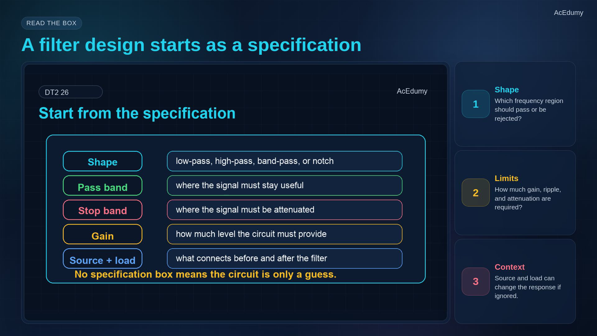
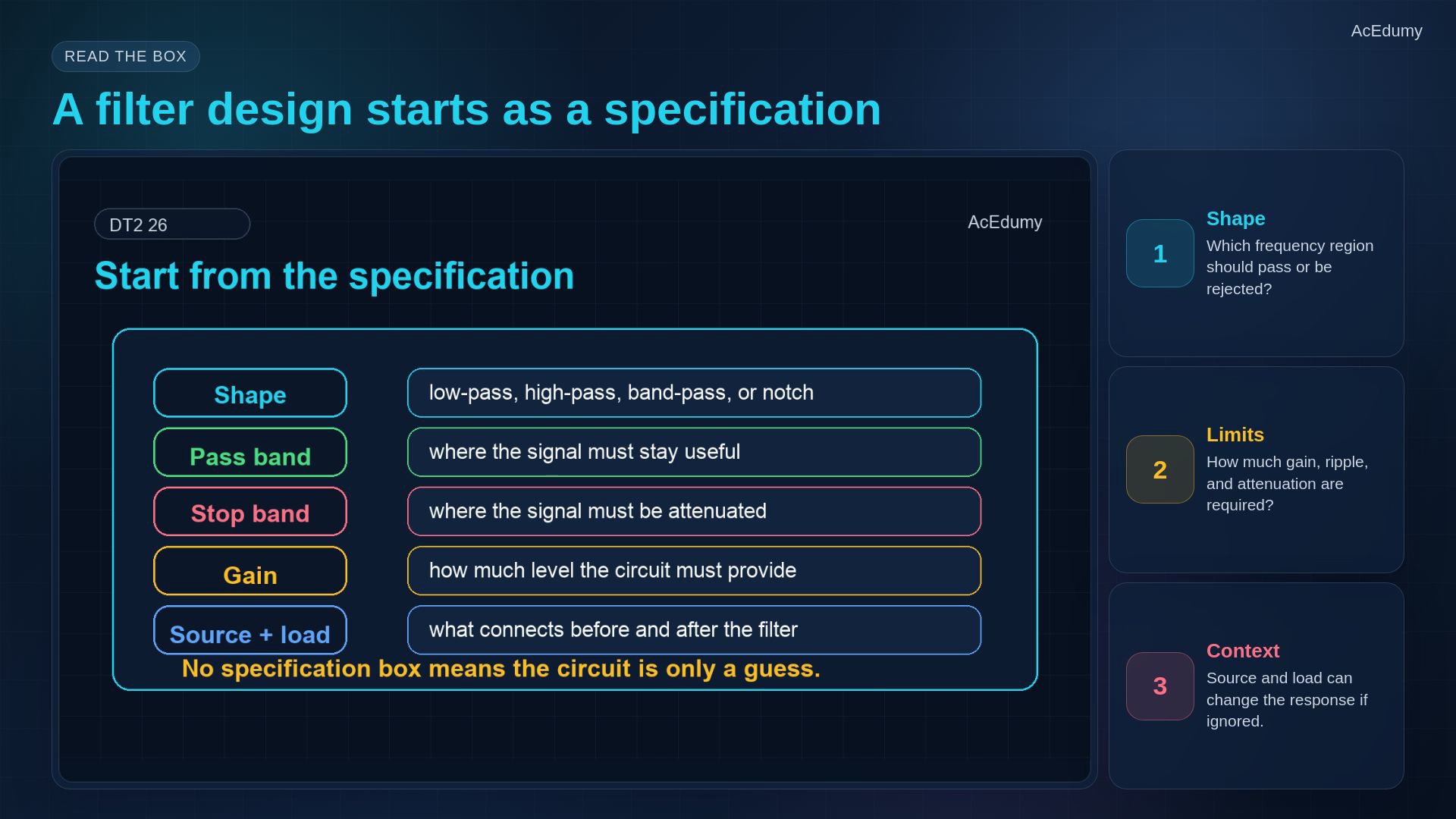
Original-video reference. Five roles use reviewed alternative cards; workflow diagrams are illustrative, not tested circuit schematics. Equations and operating assumptions appear in the notebook.
Start with a written specification, not with a favorite circuit.
Choose low-pass, high-pass, band-pass or band-reject behavior.
Mark passband, stopband, transition region and the amplitude reference.
Include required gain, source impedance, load, ripple and attenuation limits.
Also state signal amplitude, supplies and operating conditions before selecting components.
Narration transcript
A filter design starts with a specification box. First identify the shape. Then mark the pass band, stop band, and transition region. Add the required gain, the source resistance, the load, and any limit on ripple or attenuation. Without this box, the circuit is just a guess.
3. Keep units and overall edge definitions consistent
Original-video reference. Five roles use reviewed alternative cards; workflow diagrams are illustrative, not tested circuit schematics. Equations and operating assumptions appear in the notebook.
Define frequency targets for the complete response.
State the cutoff convention and its reference magnitude; not every specified edge is a half-power point.
For a standard second-order band model with the stated relative edges:
$\displaystyle Q=\frac{\omega _{0}}{\omega _{2}-\omega _{1}}$
Hertz and angular frequency both work in formulas and measurements when converted consistently:
$\displaystyle \omega =2\pi f$
Narration transcript
The frequency targets come next. For a simple edge, name the cutoff frequency. For a middle-band filter, name the lower edge, upper edge, center frequency, bandwidth, and Q. Keep the units consistent: hertz for measurement, angular frequency for formulas, and log frequency for Bode plots.
4. Choose order for the specified response family
Original-video reference. Five roles use reviewed alternative cards; workflow diagrams are illustrative, not tested circuit schematics. Equations and operating assumptions appear in the notebook.
Compare filter order within a specified response family and edge convention.
A first-order all-pole low-pass has a gentle far-out roll-off.
For an all-pole low-pass of order N the far high-frequency asymptote is:
$\displaystyle G_{\mathrm{dB}}\left(\omega \right)\approx -20N \log _{10}\left(\frac{\omega }{\omega _{c}}\right)$
A fourth-order real low-pass can be factored into two suitable second-order sections, not necessarily identical sections.
Higher order adds design constraints; sensitivity depends on pole quality factors, topology and component choices, not order alone.
Narration transcript
Order controls how aggressively the filter separates pass band from stop band. First order is gentle. Second order is sharper. Fourth order can be split into two second-order sections. The higher the order, the more stages and the more sensitivity you must manage.
5. Preserve poles and zeros across sectioning
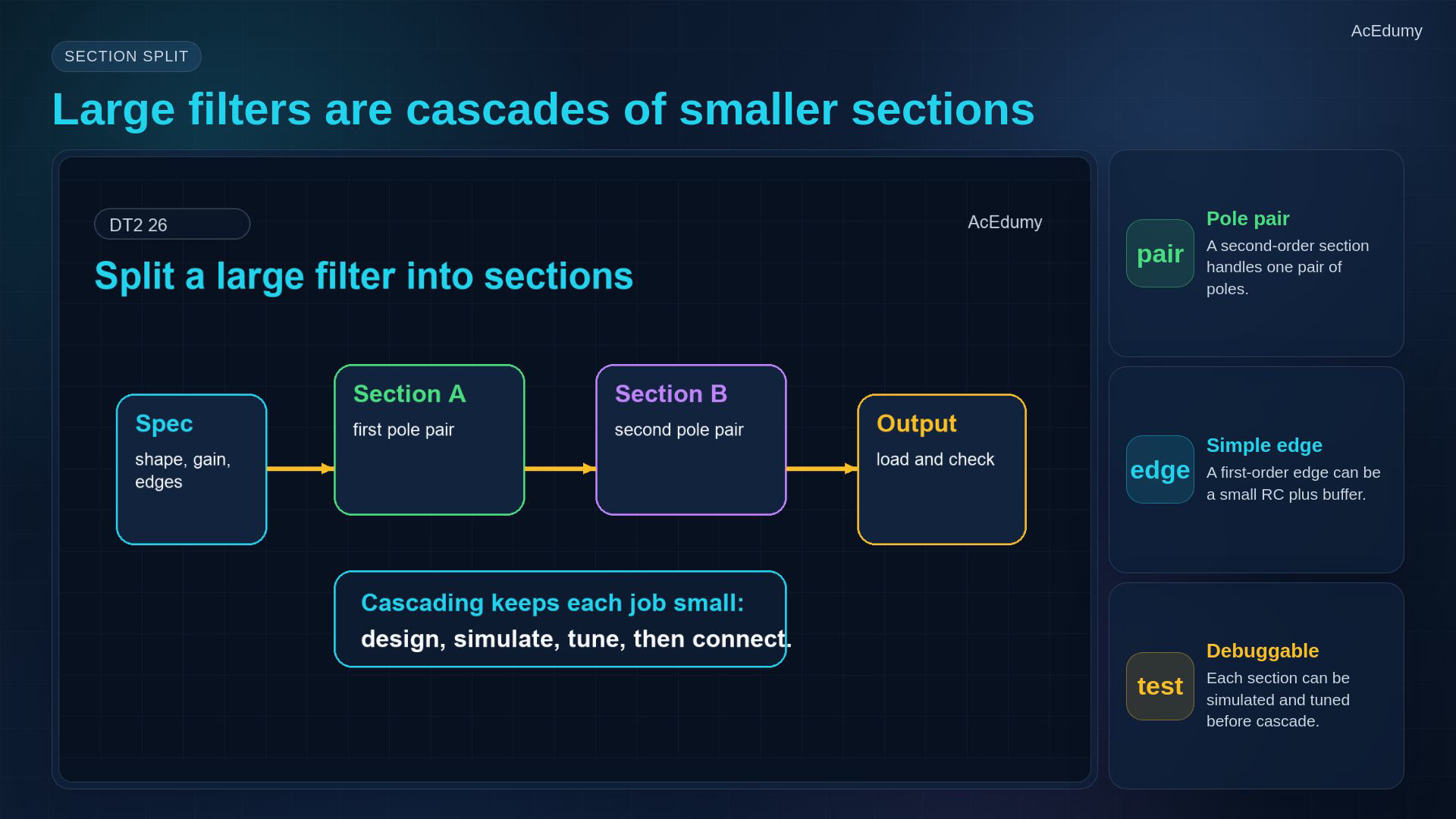
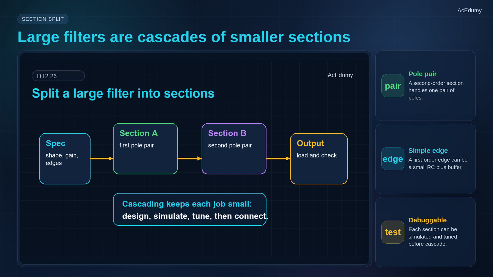
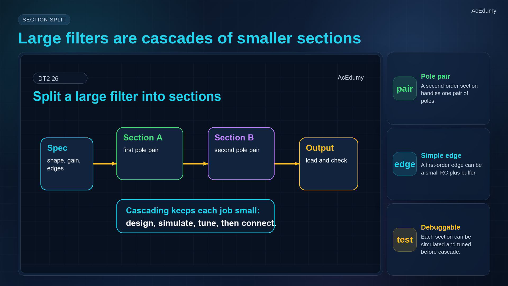
Original-video reference. Five roles use reviewed alternative cards; workflow diagrams are illustrative, not tested circuit schematics. Equations and operating assumptions appear in the notebook.
Implement the required response using manageable sections.
An ideal unloaded cascade multiplies complex section responses:
$\displaystyle H\left(s\right)=H_{1}\left(s\right) H_{2}\left(s\right)$
Assign zeros as well as poles; a second-order denominator can be written as:
$\displaystyle D_{i}\left(s\right)=s^{2}+\left(\frac{\omega _{i}}{Q_{i}}\right)s+\omega _{i}^{2}$
Preserve gain and phase while tuning sections; recheck the complete loaded response afterward.
Narration transcript
A large active filter is usually not one giant circuit. It is a cascade of smaller sections. Each section handles one pair of poles, or one simple edge. This makes the design easier to tune, easier to simulate, and easier to debug.
6. Choose topology with stability and sensitivity checks
Original-video reference. Five roles use reviewed alternative cards; workflow diagrams are illustrative, not tested circuit schematics. Equations and operating assumptions appear in the notebook.
Choose a topology that can realize the required poles, zeros and gain.
Sallen–Key is one common voltage-mode second-order topology; component ratios and gain affect its response.
Multiple-feedback is an inverting option; its suitability for the required band-pass quality factor needs calculation.
Neither topology is universally superior; compare sensitivity, noise, input impedance and op-amp loop stability.
Narration transcript
After the order is known, choose a topology. Sallen-Key is common for voltage-mode second-order sections. Multiple-feedback forms are useful when an inverting structure or tighter band-pass behavior is wanted. The topology is not the goal; it is the physical way to realize the chosen response.
7. Balance gain, headroom and input-referred noise
Original-video reference. Five roles use reviewed alternative cards; workflow diagrams are illustrative, not tested circuit schematics. Equations and operating assumptions appear in the notebook.
Allocate gain with each section's selectivity and signal swing in mind.
Qualify the source's noise shorthand; enough early low-noise gain can reduce later input-referred noise, while large unwanted signals can cause clipping.
Check gain, noise and headroom together; a three-block example has total voltage gain:
$\displaystyle K=1.5\times 1.5\times 2=4.5$
Narration transcript
Do not place all gain in the most sensitive section unless you have a reason. Distribute gain so the op-amp has headroom, the signal does not clip, and noise is not amplified too early. A clean block diagram often prevents a messy circuit.
8. Recalculate after scaling and component rounding
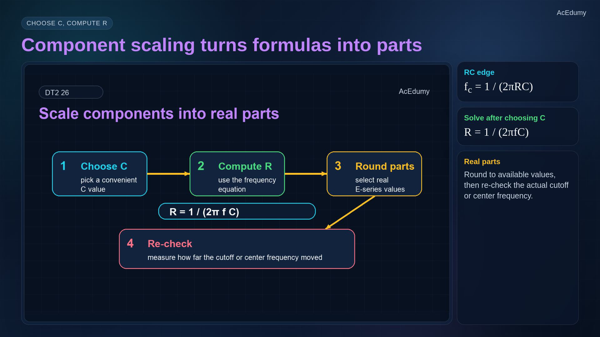
Original-video reference. Five roles use reviewed alternative cards; workflow diagrams are illustrative, not tested circuit schematics. Equations and operating assumptions appear in the notebook.
Choose practical component scales without changing the required response.
For an illustrative ideal single-pole RC corner only, choose C then calculate:
$\displaystyle R=\frac{1}{2\pi f_{c} C}$
After rounding parts, recalculate the actual corner:
$\displaystyle f_{c}=\frac{1}{2\pi R C}$
Second-order topology equations also control quality factor and gain; a single RC formula is not a complete design.
Narration transcript
Component scaling is the practical arithmetic step. Choose convenient capacitor values, then compute resistor values. After that, round to real component series values and check how far the cutoff or center frequency moved. Good design is not just solving a formula; it is landing on parts you can buy.
9. Model source and interstage loading
Original-video reference. Five roles use reviewed alternative cards; workflow diagrams are illustrative, not tested circuit schematics. Equations and operating assumptions appear in the notebook.
Source and load impedances can alter the designed response.
A simple Thevenin source feeding a finite input gives a complex voltage divider:
$\displaystyle \frac{V_{\mathrm{in}}}{V_{s}}=\frac{Z_{\mathrm{in}}}{Z_{s}+Z_{\mathrm{in}}}$
Buffers reduce interaction but still have finite current, bandwidth and stability limits; they are not galvanic isolation.
Narration transcript
Loading can quietly change the filter. The source can load the first stage, one stage can load the next, and the output load can change the final response. Buffers and active stages reduce this interaction, but every op-amp still has finite output current and bandwidth.
10. Verify the complete circuit against specifications
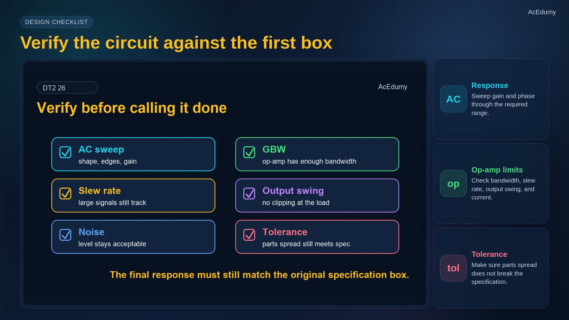
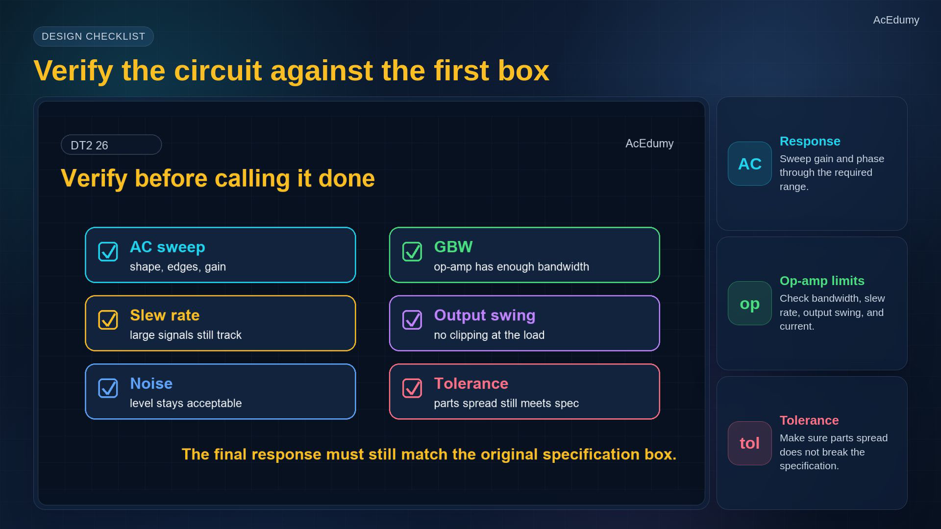
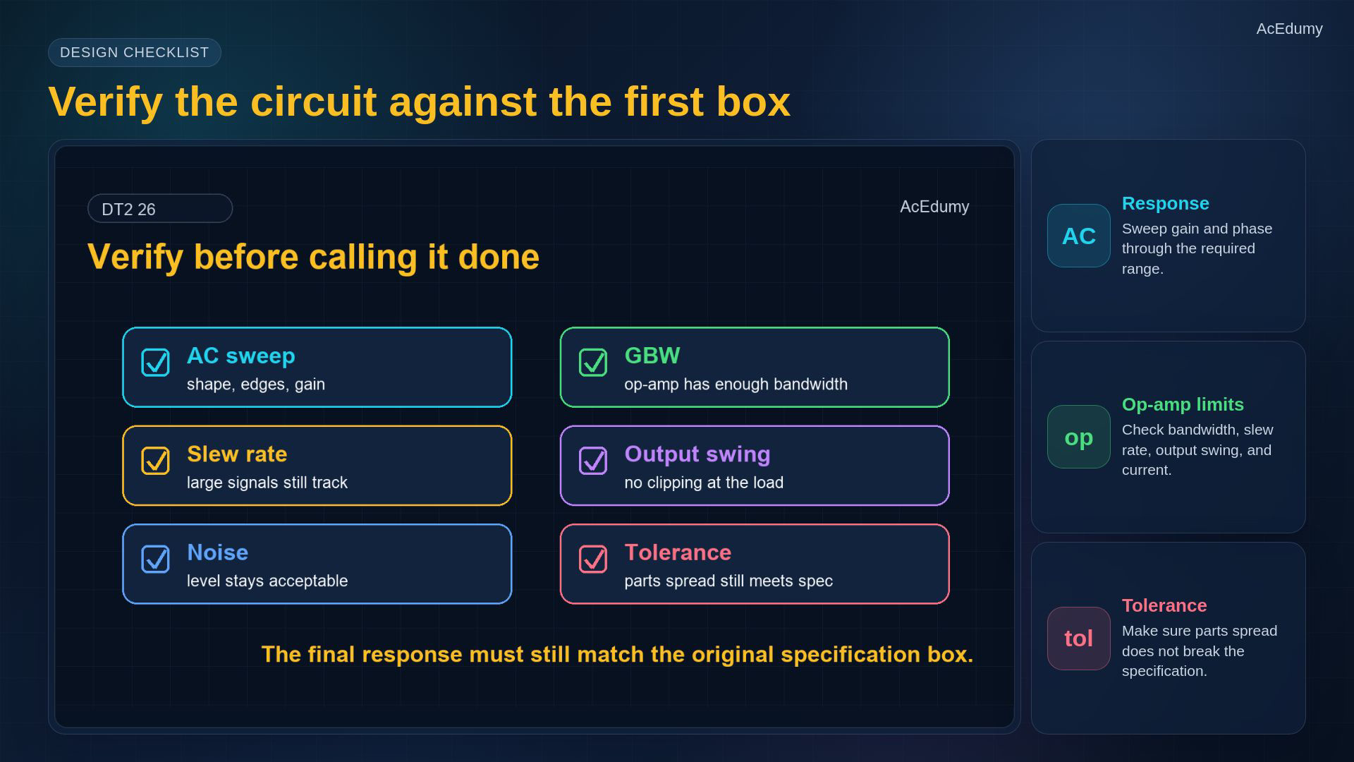
Original-video reference. Five roles use reviewed alternative cards; workflow diagrams are illustrative, not tested circuit schematics. Equations and operating assumptions appear in the notebook.
Use a verification checklist; printed check marks are not completed hardware tests.
Minimum sinusoidal-output slew requirement, alongside small-signal and other checks:
$\displaystyle S_{\mathrm{min}}=2\pi f V_{\mathrm{pk}}$
Compare the nonideal simulated and measured response against the original specifications, including noise and tolerance.
Narration transcript
Before calling the design finished, run a verification checklist. Check the AC sweep, the gain-bandwidth product, slew rate, output swing, noise, and component tolerance. Then inspect whether the response still meets the original specification box.
11. Summarize the design-to-verification chain
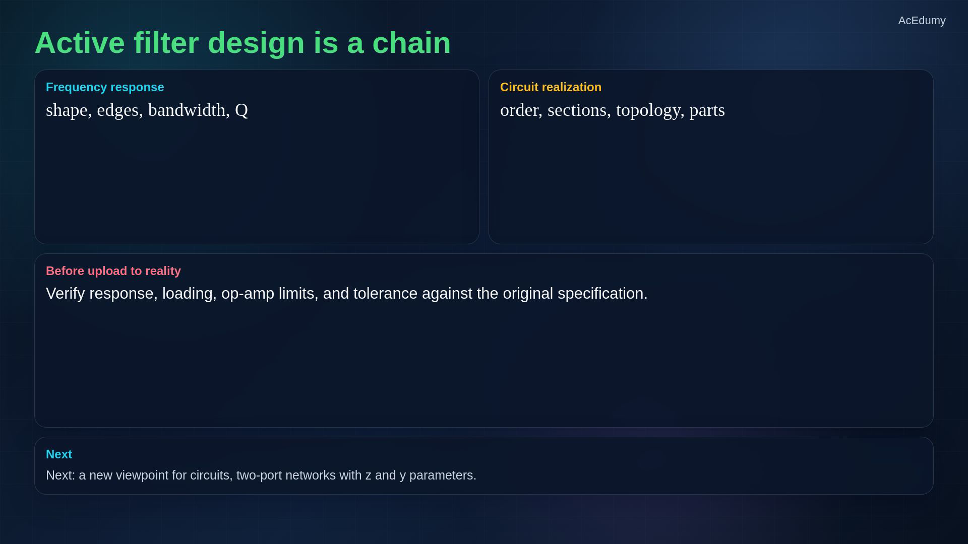
Original-video reference. Five roles use reviewed alternative cards; workflow diagrams are illustrative, not tested circuit schematics. Equations and operating assumptions appear in the notebook.
Summary: design is an iterative specification-to-verification process.
Follow the response targets through order, sections, topology, gain allocation, scaling and verification.
A plausible block diagram becomes a buildable circuit only after its electrical limits are checked.
Next, describe two-port networks using impedance and admittance parameters with stated port-current conventions.
Narration transcript
Summary. Active filter design is a chain: specification, frequency targets, order, section split, topology, component scaling, and verification. That chain turns frequency-response intuition into a buildable circuit. Next, we will change viewpoint and describe circuits as two-port networks using z and y parameters.