Circuit Theory 2 · Active low-pass and high-pass filters

#24 Ideal inverting RC topologies, signed gain, cutoff and practical limits

Derive the inverting active RC responses, choose gain and cutoff components, and distinguish specific passive divider examples from general passivity.

Question

Original English video reference showing an active filter circuit, component design, practical limits or the low-pass and high-pass summary. — The low-pass and high-pass equation roles reuse their corresponding circuit references; the curve-comparison role uses the original summary card. Use the notebook equations for quantitative gain and cutoff values.

Derive the ideal inverting active low-pass and high-pass transfer functions and design the low-pass example for 1 kHz, C=10 nF and signed gain -2. Use positive constant components and an ideal op-amp in stable negative feedback, linear operation, adequate power supplies and initially relaxed capacitors. Voltages share the shown ground reference. R_i denotes the source's input resistor R_in, R_f the feedback resistor, V_i the ideal source voltage and V_o the output. The noninverting input is grounded; the inverting node is a virtual ground under these assumptions, not a physical ground connection. Ideal op-amp terminal input currents vanish, while current through the external input and feedback components does not. The opening first recalls the four previously taught passive output choices: RC capacitor-output low-pass, RC resistor-output high-pass, series RLC resistor-output band-pass, and series RLC combined-reactance output band-reject. Their ideal voltage-transfer magnitudes do not exceed one. Read the following passive-gain shorthand within that immediate context. It is not a general passivity theorem: an ideal voltage-driven passive series RLC with capacitor output has resonant voltage magnitude Q times the input and can exceed one without producing average real power. For normalized frequency x and positive Q, the four earlier transfers are 1/(1+jx), jx/(1+jx), 1/[1+jQ(x-1/x)], and jQ(x-1/x)/[1+jQ(x-1/x)]; each has magnitude at most one. In the counterexample with capacitor output, at resonance the reactive voltages cancel in the series sum but can individually be large. Source real power still equals resistor dissipation. Voltage magnification and power gain are different quantities. This explicit scope preserves the original recording and does not replace a spoken number or equation. For the low-pass circuit, R_f and C connect between the same two nodes: the inverting node and the output. The feedback impedance is Z_f=R_f/(1+sR_fC). KCL with virtual ground gives V_i/R_i=-V_o/Z_f, hence H_L(s)=V_o/V_i=-(R_f/R_i)/(1+sR_fC). Its signed DC pass-band gain is A_v=-R_f/R_i. The feedback time constant is τ_L=R_fC, angular cutoff ω_L=1/(R_fC) and ordinary cutoff f_L=1/(2πR_fC). The minus sign means inversion; it is not a negative magnitude. At low frequency the capacitor branch is nearly open, while at high frequency its decreasing impedance reduces feedback impedance and signal gain. For the high-pass circuit, C is in series with R_i in the input path and R_f alone provides feedback. The input impedance is R_i+1/(sC); H_H(s)=-(R_f/R_i)sR_iC/(1+sR_iC). Here τ_H=R_iC, ω_H=1/(R_iC) and f_H=1/(2πR_iC). The signed high-frequency gain approaches A_v=-R_f/R_i in the ideal model. Statements that the signal reaches the inverting node refer to input current and feedback action. The node voltage remains approximately zero; it does not become the source voltage. The practical high-frequency pass band lies inside the op-amp operating range, not at infinite frequency. For either response the magnitude at its corner is |A_v|/sqrt(2), which is about -3.0103 dB relative to its pass band. An absolute -3 dB voltage-gain level applies only when the pass-band magnitude is one. The plotted legacy curves use linear magnitude geometry while labeling their vertical axes in dB; those three curve frames are excluded from notebook references. For quantitative results use these equations. At positive frequency with the e^(jωt) convention, the inverting low-pass corner phase is +135 degrees and the inverting high-pass corner phase is -135 degrees on the principal branch. Their poles lie on the negative real axis for positive R,C. Rejection describes asymptotic attenuation, not a sharp rectangular band. At fixed R_f,C, choose R_i for low-pass gain without changing its ideal cutoff. At fixed R_i,C, choose R_f for high-pass gain. Changing the resistor in the relevant time constant changes cutoff as well. The nominal low-pass example gives R_f=15915.494309 ohms and R_i=7957.747155 ohms, approximately 15.9 and 7.96 kilohms. The spoken gain is minus two. If rounded standard resistor values are selected, recalculate both cutoff and ratio. The original design graphic additionally gives a high-pass example at 100 Hz and 100 nF with R_i about15.9 kilohms; that is a separate illustrated example, not the spoken one-kilohertz low-pass case. An op-amp can reduce the effect of a following stage by providing low closed-loop output impedance within its limits. These inverting circuits still load the preceding source through their finite input impedance: R_i for the ideal low-pass, and R_i+1/(jωC) for the high-pass. Infinite op-amp terminal input impedance does not imply an infinite stage input impedance. If a source resistance is significant, include it in the actual network. Check open-loop gain, feedback stability, gain-bandwidth, input common-mode range, output current and load, signal swing, slew rate, component tolerances and bias-current paths against the actual device. The usable output swing is normally smaller than the supply-rail span. The ideal equations assume sufficient margin, and gain greater than unity requires energy from the power supplies. The selected original low-pass image has a caption partly covering the ground symbol, but its grounded noninverting connection and both common feedback nodes remain identifiable. The op-amp-role card has text crossing a small diagram border, and the practical-limits caption extends beyond its box without losing the sentence. These layout limitations do not change the equations. The equation roles use the corresponding unchanged topology frames, and the comparison role uses the unchanged summary card, so no defective quantitative curve is used. The summary's next-topic card mentions Butterworth additionally; the spoken recap is limited to active middle-band filtering.

Written solution and narration transcript(shows the full solution)

Below are all the lines written in the notebook together with the full narration transcript.

1. Compare the previous passive examples with active filters
The low-pass and high-pass equation roles reuse their corresponding circuit references; the curve-comparison role uses the original summary card. Use the notebook equations for quantitative gain and cutoff values.
Recall the four passive filter examples.
Those particular outputs have magnitude at most one; passivity alone does not forbid voltage magnification.
Use an op-amp to control gain and reduce interaction between stages.
Narration transcript
Passive filters gave us the four basic shapes: low-pass, high-pass, band-pass, and band-reject. But passive filters cannot create voltage gain, and their response can change when the next stage loads them. Active filters add an op-amp so the frequency selection and the signal gain can be designed more deliberately.
2. State gain, isolation and operating limits
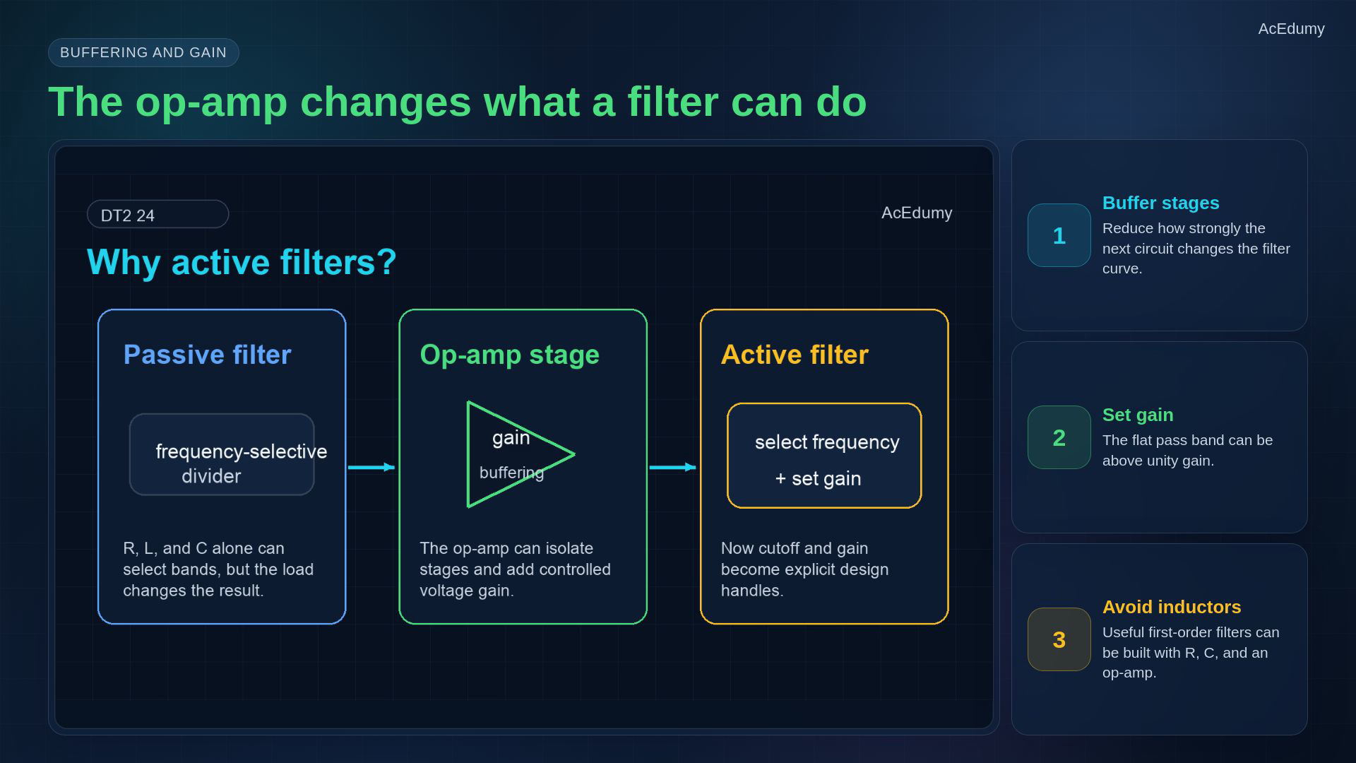
The low-pass and high-pass equation roles reuse their corresponding circuit references; the curve-comparison role uses the original summary card. Use the notebook equations for quantitative gain and cutoff values.
Three roles for the op-amp
Reduce the effect of the following load within the operating range.
The pass-band voltage magnitude may exceed unity.
Build first-order responses with resistors and capacitors.
Narration transcript
The op-amp does three useful jobs. First, it can isolate one stage from the next. Second, it can provide voltage gain, so the pass band does not have to be below unity. Third, it lets us build clean first-order filter blocks using resistors and capacitors instead of inductors.
3. Place parallel R and C in negative feedback
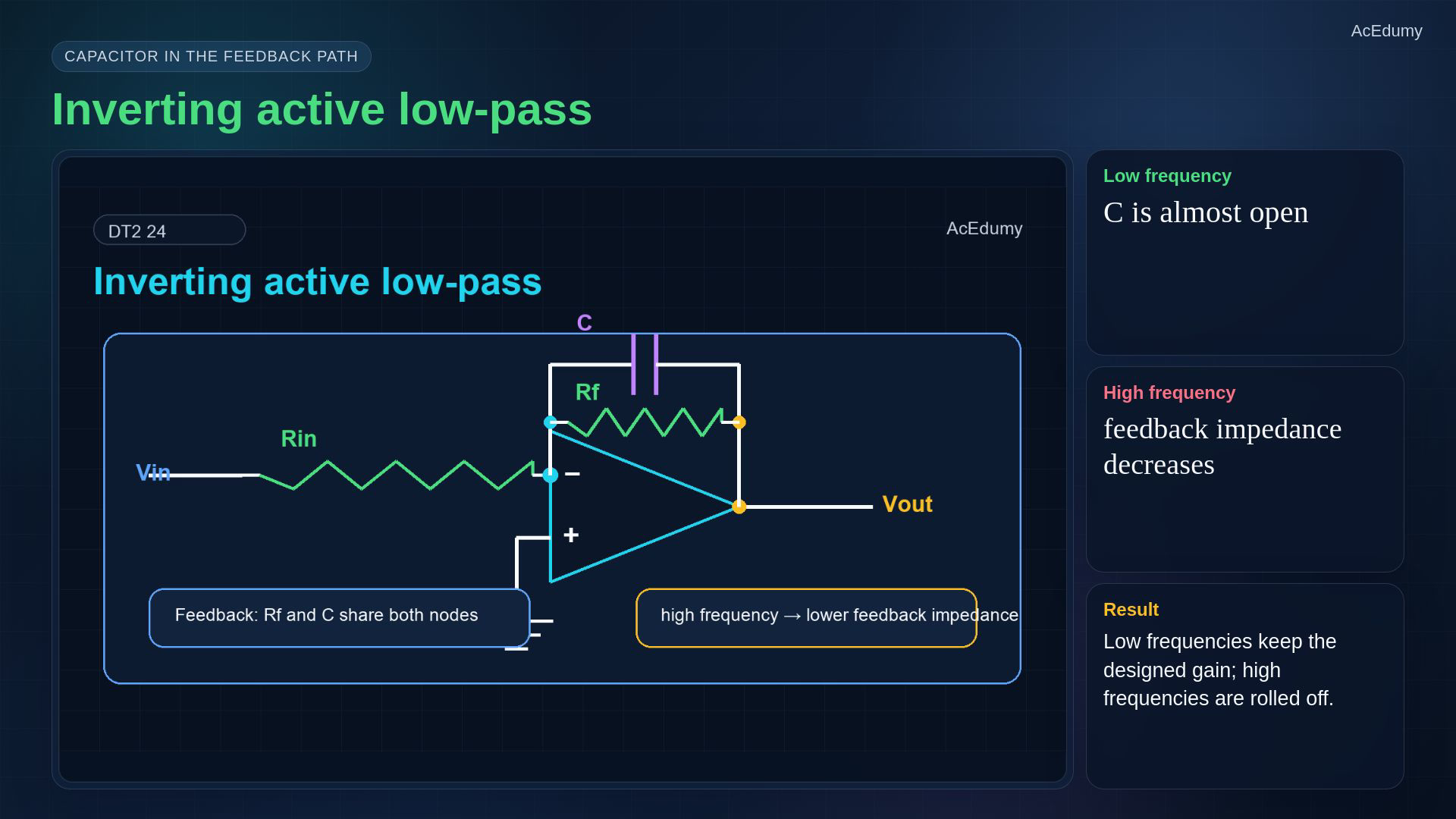
The low-pass and high-pass equation roles reuse their corresponding circuit references; the curve-comparison role uses the original summary card. Use the notebook equations for quantitative gain and cutoff values.
Use an inverting low-pass circuit.
Ideal input current:
$\displaystyle I_{i} =\frac{ V_{i}}{R_{i}}$
Parallel feedback impedance:
$\displaystyle Z_{f}\left(s\right) =\frac{ R_{f}}{1 + s R_{f} C}$
At low frequency, the capacitor branch is nearly open.
Low-pass transfer:
$\displaystyle H_{L}\left(s\right) = -\frac{\frac{R_{f}}{R_{i}}}{1 + s R_{f} C}$
Narration transcript
Start with an inverting active low-pass filter. The input resistor feeds the inverting node. In the feedback path, a resistor is placed in parallel with a capacitor. At low frequency the capacitor is almost open, so the feedback is mostly through the resistor. At high frequency the capacitor reduces the feedback impedance, so the closed-loop gain falls.
4. Separate low-pass gain and time constant
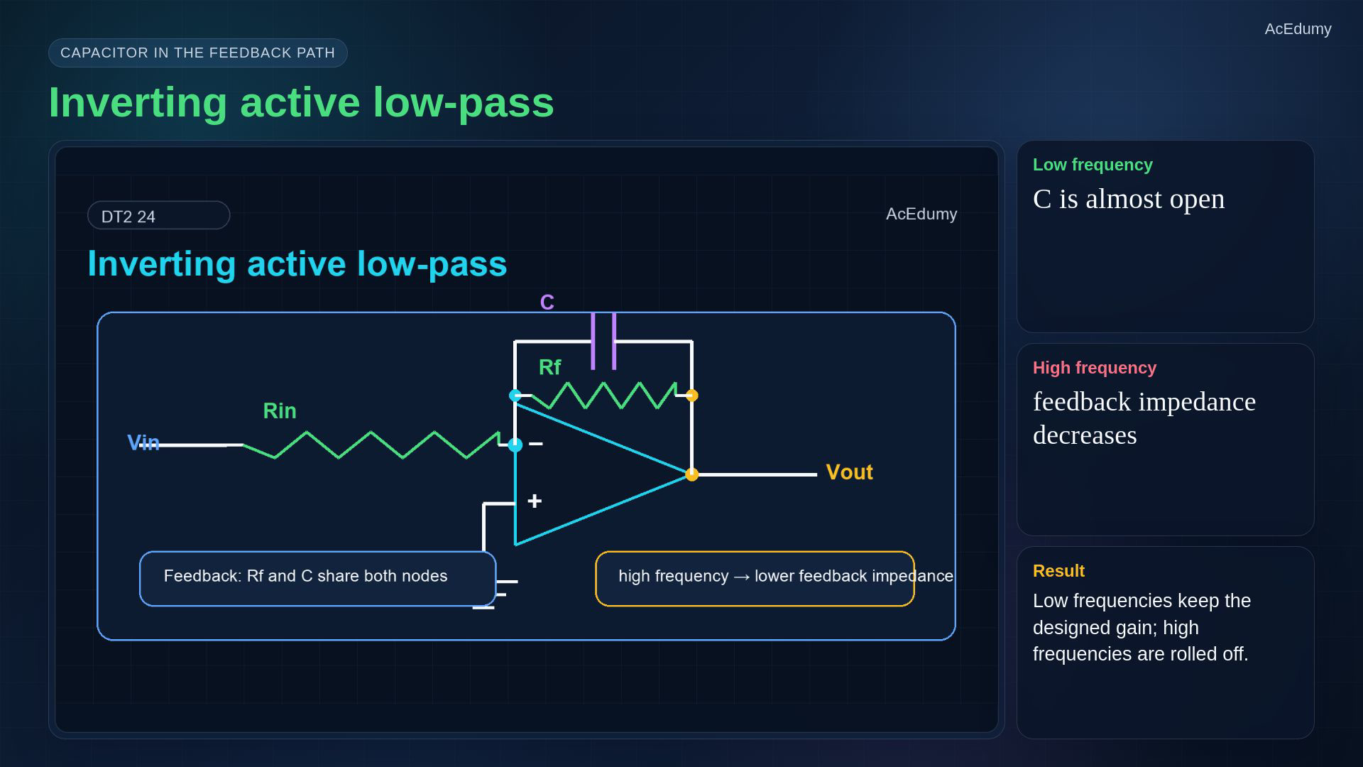
The low-pass and high-pass equation roles reuse their corresponding circuit references; the curve-comparison role uses the original summary card. Use the notebook equations for quantitative gain and cutoff values.
Signed pass-band gain:
$\displaystyle A_{v} = -\frac{R_{f}}{R_{i}}$
Feedback time constant:
$\displaystyle \tau _{L} = R_{f} C$
Low-pass cutoffs:
$\displaystyle \omega _{L} =\frac{ 1}{R_{f} C}, f_{L} =\frac{ 1}{2\pi R_{f} C}$
Narration transcript
For this low-pass form, the pass-band gain is set by the resistor ratio, minus R f over R in. The cutoff comes from the feedback time constant R f times C. So the angular cutoff is one over R f C, and the hertz cutoff is one over two pi R f C.
5. Place C in series with the input resistor
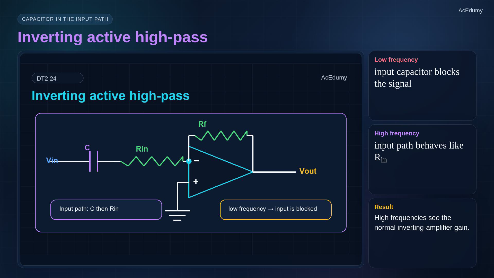
The low-pass and high-pass equation roles reuse their corresponding circuit references; the curve-comparison role uses the original summary card. Use the notebook equations for quantitative gain and cutoff values.
Move C into series with the input resistor.
At low frequency the input impedance is large.
High-pass transfer:
$\displaystyle H_{H}\left(s\right) = -\frac{\left(\frac{R_{f}}{R_{i}}\right) s R_{i} C}{1 + s R_{i} C}$
Narration transcript
The active high-pass version moves the capacitor into the input path. At low frequency the input capacitor blocks the signal, so the output is small. At high frequency the capacitor behaves almost like a short, and the circuit becomes an ordinary inverting amplifier.
6. Use the high-pass input time constant
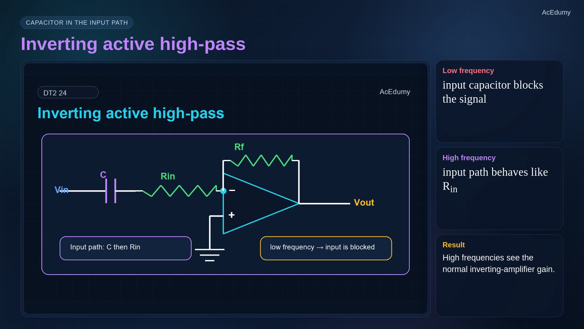
The low-pass and high-pass equation roles reuse their corresponding circuit references; the curve-comparison role uses the original summary card. Use the notebook equations for quantitative gain and cutoff values.
Signed high-frequency gain:
$\displaystyle A_{v} = -\frac{R_{f}}{R_{i}}$
Input time constant:
$\displaystyle \tau _{H} = R_{i} C$
Increasing signal current does not make the virtual-ground node follow the input voltage.
Narration transcript
For the high-pass form, the high-frequency gain is again minus R f over R in. The cutoff now comes from the input time constant R in times C. Below cutoff the input path is weak; above cutoff the input reaches the inverting node efficiently.
7. Compare normalized shapes and chosen passband gain
The low-pass and high-pass equation roles reuse their corresponding circuit references; the curve-comparison role uses the original summary card. Use the notebook equations for quantitative gain and cutoff values.
Compare the familiar normalized low-pass and high-pass shapes.
The pass-band height is set by the magnitude of the resistor ratio.
Choose the gain resistor without changing the cutoff time constant.
Narration transcript
The magnitude curves look familiar, but there is one important difference from passive R C filters. The flat part of the curve can sit at a chosen gain, not just at zero decibels. The op-amp gives us a design handle for gain, while the resistor-capacitor product gives us the corner frequency.
8. Calculate nominal cutoff and resistor ratio
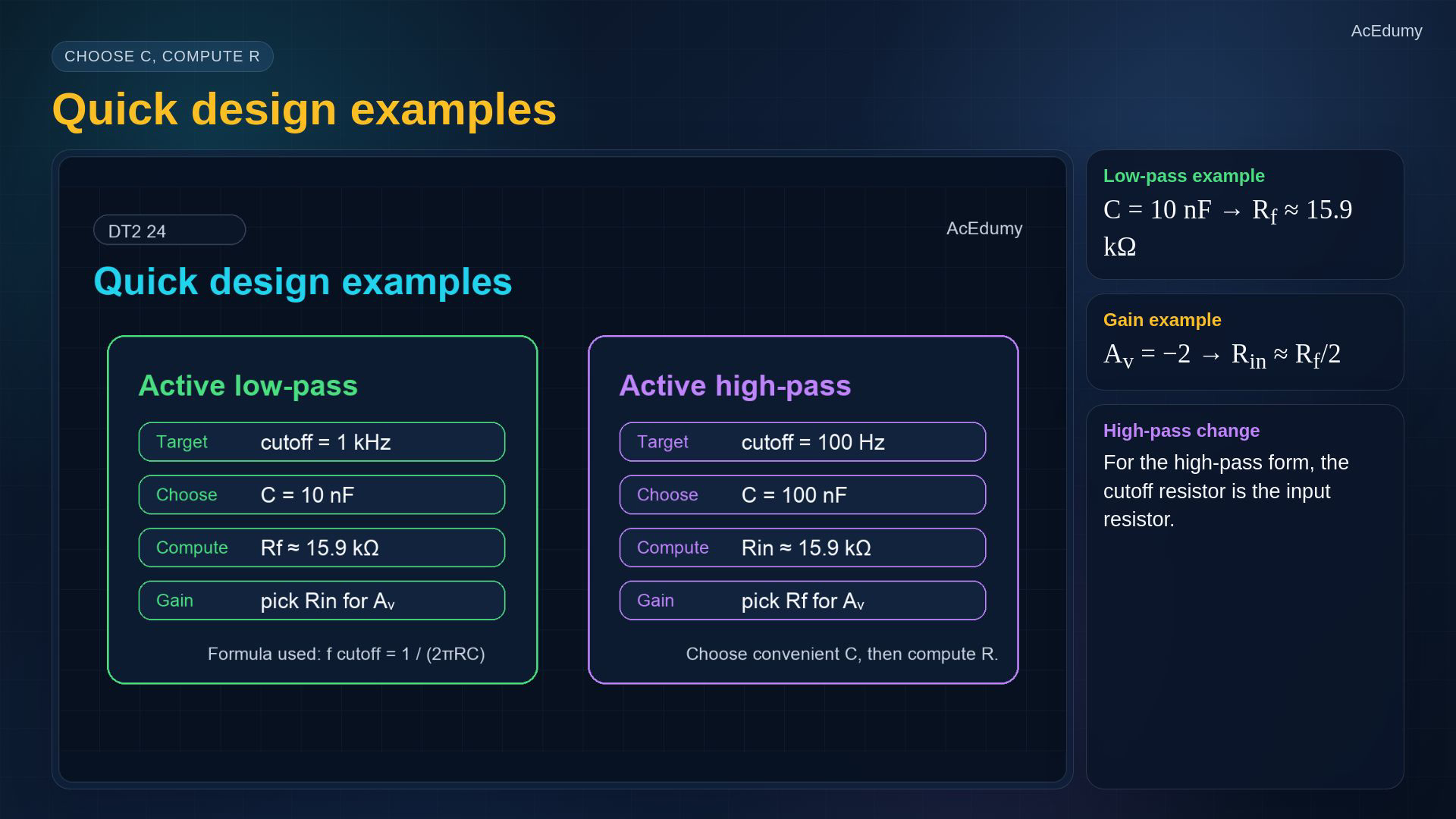
The low-pass and high-pass equation roles reuse their corresponding circuit references; the curve-comparison role uses the original summary card. Use the notebook equations for quantitative gain and cutoff values.
Design the nominal low-pass example.
Choose a one-kilohertz cutoff and ten nanofarads.
Feedback resistor:
$\displaystyle R_{f} =\frac{ 1}{2\pi f_{L} C}$
For signed gain minus two:
$\displaystyle R_{i} =\frac{ R_{f}}{2}$
For high-pass design, the input resistor sets cutoff.
Narration transcript
A quick design example. For an active low-pass cutoff of one kilohertz, choose C equal to ten nanofarads. Then R f is about fifteen point nine kilohms. If you want a pass-band gain of minus two, choose R in about half of R f. The same workflow works for high-pass filters, but the cutoff resistor is the input resistor.
9. Check bandwidth, slew, swing and load
The low-pass and high-pass equation roles reuse their corresponding circuit references; the curve-comparison role uses the original summary card. Use the notebook equations for quantitative gain and cutoff values.
Check the limits of the ideal model.
Open-loop gain and bandwidth must support the desired closed-loop response.
Large fast signals can be limited by slew rate.
Output swing must remain inside the usable supply and load limits.
Resistor and capacitor tolerances shift the actual cutoff.
Narration transcript
Active filters are not magic. The op-amp must have enough gain-bandwidth at the frequencies you care about. Large fast signals can hit the slew-rate limit. The output cannot exceed the supply rails. And real resistor and capacitor tolerances shift the cutoff from the ideal value.
10. Apply the design checks
The low-pass and high-pass equation roles reuse their corresponding circuit references; the curve-comparison role uses the original summary card. Use the notebook equations for quantitative gain and cutoff values.
Apply the design recipe.
Choose low-pass or high-pass.
Angular and ordinary cutoff:
$\displaystyle \omega _{c} = 2\pi f_{c}$
Choose a convenient capacitor.
Calculate the resistor in the relevant time constant.
Set the signed pass-band gain through the resistor ratio.
Check bandwidth, slew rate, swing and load.
Narration transcript
The design recipe is simple. Choose the filter shape. Choose the cutoff frequency. Pick a convenient capacitor. Compute the resistor that sets the time constant. Then choose the resistor ratio that sets pass-band gain. Finally, check the op-amp data sheet against bandwidth, slew rate, signal swing, and load.
11. Summarize the inverting RC filter blocks
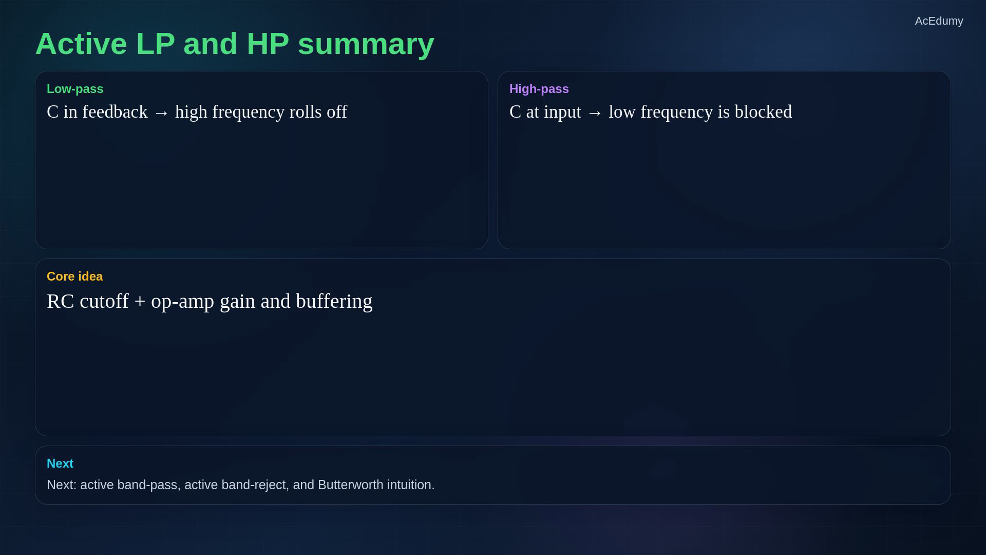
The low-pass and high-pass equation roles reuse their corresponding circuit references; the curve-comparison role uses the original summary card. Use the notebook equations for quantitative gain and cutoff values.
Active RC filter summary
Combine a first-order response with op-amp gain and reduced stage interaction.
Low-pass uses a capacitor parallel to the feedback resistor.
High-pass uses a capacitor in series with the input resistor.
Next apply active filtering to middle-band responses.
Narration transcript
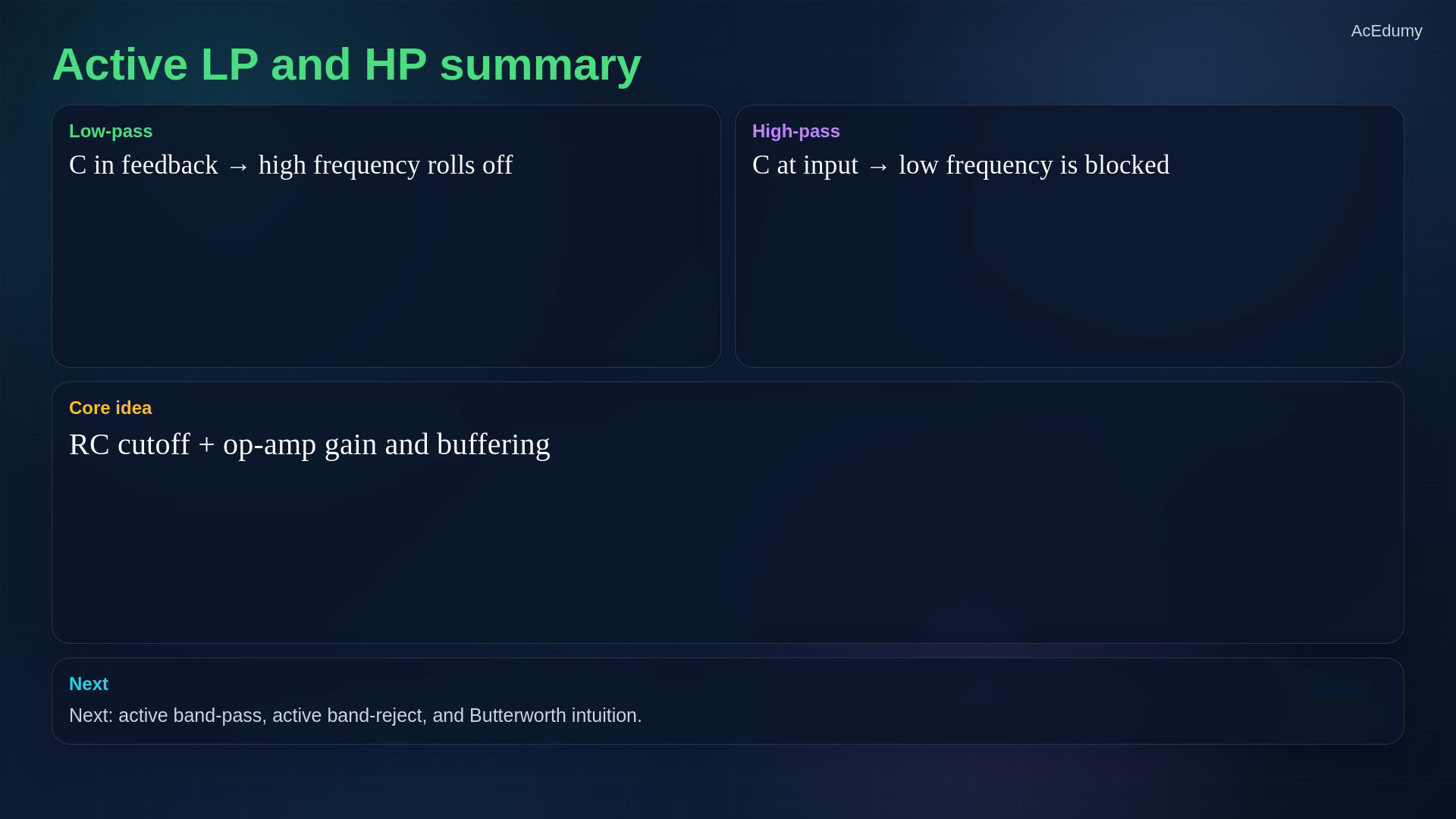
Summary. An active low-pass or high-pass filter combines a first-order R C frequency response with op-amp gain and buffering. Low-pass puts the capacitor in the feedback path. High-pass puts the capacitor in the input path. Next, we will use the same active-filter idea to build middle-band behavior: active band-pass and band-reject filters.