Circuit Theory 2 · Band-pass filters, resonance and Q

#22 Resistor-output series RLC, relative cutoffs, normalized peak, loss and loading

Derive the series RLC band-pass response, calculate its half-power bandwidth and distinguish a sharper Q shape from a larger peak gain.

Question

Unmodified original English video reference showing the middle pass band, equal-height Q curves, reactance cancellation, practical checks or the resonance and bandwidth formulas. — The Q curves illustrate relative shape and equal peak height. Read their axes qualitatively; use the notebook formulas for exact cutoff values. Resonance and summary cards are reused for roles whose original plot or circuit reference is unsuitable.

Derive the series RLC band-pass transfer with the output taken across R, identify its relative half-power cutoffs and calculate the example. Assume positive constant R,L,C, an ideal voltage source, negligible added component loss, an unloaded resistor output and sinusoidal steady state. Use the same peak or RMS phasor convention throughout, with e^(jωt) and positive frequency. The output voltage is across both terminals of R with the passive current reference; it is not the grounded end of R measured against ground. The impedances add in series: Z=R+j(ωL−1/(ωC)), I=V_in/Z and H(jω)=V_R/V_in=R/Z. The low- and high-frequency statements describe limiting attenuation, not perfect rejection at every finite frequency outside an ideal rectangular window. At ω_0=1/√(LC), the reactive terms cancel exactly in this ideal model and H(jω_0)=1. The reference's “almost purely resistive” allows practical imperfections. Cancellation does not remove L and C or stop their stored-energy exchange. In the reactance card X_L=ωL and X_C=1/(ωC) are positive magnitudes; the actual capacitor impedance is −jX_C. In the Q narration, “a tall, narrow, selective response” describes a sharply peaked shape. The same source explains the peak as voltage division, labels its Q graphic as narrow versus broad, and draws both curves with the same peak. Here tall must not be interpreted as increasing absolute peak voltage with Q: the normalized resistor-output peak remains exactly one for every positive Q. A larger Q at fixed center frequency makes the bandwidth narrower and the peak sharper relative to its width. This interpretation does not change a spoken number, sign, equation, sound or timing. The Q graphic is a qualitative shape reference with compressed log-frequency and logarithmic magnitude geometry; its generic axis labels and unnumbered tick positions are not a calibrated linear-gain/frequency scale. Its equal-height peaks are the relevant visual feature. Let x=ω/ω_0. Then H=1/[1+jQ(x−1/x)], Q=ω_0L/R=√(L/C)/R. The magnitude is no greater than one and equals one only at resonance for finite positive parameters. Resistor output and the ideal voltage-driven model matter: voltages across reactive elements can exceed the input, and passivity alone does not prohibit reactive voltage magnification. Thus the narration's passive-peak explanation is scoped to the stated resistor output, not a universal prohibition of passive voltage gain. The relative half-power frequencies satisfy |H|=1/√2 times the peak, equivalent to about −3.0103 dB in voltage magnitude relative to that peak. The two positive normalized roots are x_1=(√(4+1/Q²)−1/Q)/2 and x_2=(√(4+1/Q²)+1/Q)/2. They obey x_2−x_1=1/Q and x_1x_2=1. Consequently B_ω=ω_2−ω_1=R/L and B_f=f_2−f_1=B_ω/(2π), while Q=ω_0/B_ω=f_0/B_f. Keep angular frequencies in radians per second and ordinary frequencies in hertz; mixing them introduces a factor of 2π. The center is the geometric mean of the exact edges, not generally their arithmetic midpoint. The −3 dB boundary is a response threshold, not an abrupt wall. Use the common notebook equations and summary reference for exact cutoff calculations. The original response-curve graphic's plotted cutoff markers and dB ticks do not match its underlying response function, and the original series diagram marks the ground side as an output node. Those images are not used for their affected notebook roles. The reactance reference used for the circuit role is an explanation card, not a complete circuit topology diagram. No alternate topology is inferred from it. The selected same-video originals remain unmodified. The resonance frame's bottom caption is partly clipped, but its equations and reactance signs remain readable. The Q frame has a small paragraph extending beyond its box; it does not hide the equations or peak comparison. Below resonance, net impedance reactance is negative, so the resistor voltage leads the source; above resonance it lags. At resonance they are in phase. The transfer phase is the negative of the series-impedance phase and tends toward +90° and −90° at the low- and high-frequency limits. The scalar condition X_L=X_C concerns magnitudes, while the complex terms have opposite signs. For L=10 mH=0.01 H, C=100 nF=10^−7 F and R=100 Ω, ω_0 is about 31622.7766 rad/s and f_0 about 5032.9212 Hz. Q=√10 is about 3.16228, B_ω=10000 rad/s and B_f about 1591.54943 Hz. The spoken 5.03 kHz, 3.16 and 1.59 kHz are appropriately rounded values. Use the lowercase milli and nano prefixes as spoken; the original design scene's uppercase decorative kicker is not used as a units reference. Changing R at fixed ideal L,C changes Q inversely and bandwidth directly, while leaving the center frequency and normalized peak unchanged. If an additional series resistance r represents source or component loss but output remains across the designated R, the resonant voltage ratio becomes R/(R+r), and Q uses total series resistance R+r. Finite output loading can change both the effective network and its frequency response; apply the actual connection instead of treating every loss as the same resistor. A particular lossy family may change Q and peak together, but this is not a universal relationship. Positive R prevents the ideal series singularity that would arise in the undamped R=0 limit. Practical bandwidth, loading, component tolerances and operating limits must be assessed for a real implementation. Higher Q is useful for selection but can reject desired neighboring frequencies; choose it according to the required pass band.

Written solution and narration transcript(shows the full solution)

Below are all the lines written in the notebook together with the full narration transcript.

1. Select a middle frequency band
The Q curves illustrate relative shape and equal peak height. Read their axes qualitatively; use the notebook formulas for exact cutoff values. Resonance and summary cards are reused for roles whose original plot or circuit reference is unsuitable.
From low-pass and high-pass to band-pass
Keep a band around a center frequency.
Attenuate frequencies far below and far above that band.
At resonance, inductive and capacitive reactances cancel.
Narration transcript
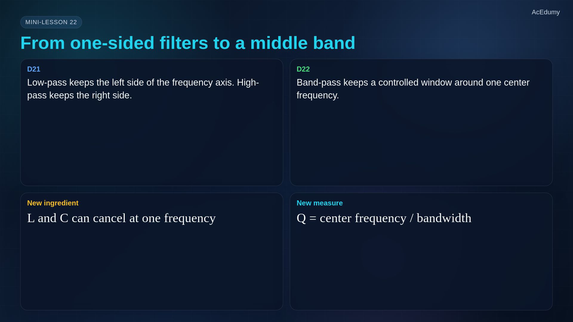
In the previous lesson, low-pass and high-pass filters kept one side of the frequency axis. Now we keep the middle. A band-pass filter rejects very low frequencies, rejects very high frequencies, and passes a band around a center frequency. The new idea is resonance: an inductor and a capacitor can cancel each other's reactance at one frequency.
2. Identify center and cutoff frequencies
The Q curves illustrate relative shape and equal peak height. Read their axes qualitatively; use the notebook formulas for exact cutoff values. Resonance and summary cards are reused for roles whose original plot or circuit reference is unsuitable.
Identify the center and two cutoff frequencies.
The center gives the peak of this response.
The two cutoffs are measured relative to the peak.
Hertz bandwidth:
$\displaystyle B_{f} = f_{2} - f_{1}$
A narrower band gives stronger frequency selection.
Narration transcript
A band-pass filter has three landmarks. The center frequency is where the response is largest. The lower and upper cutoff frequencies mark the minus-three-decibel edges. The bandwidth is the distance between those two edges. A narrow bandwidth means the filter is selective; a wide bandwidth means it is forgiving.
3. Specify the resistor output and references
The Q curves illustrate relative shape and equal peak height. Read their axes qualitatively; use the notebook formulas for exact cutoff values. Resonance and summary cards are reused for roles whose original plot or circuit reference is unsuitable.
Series RLC with output across the resistor:
$\displaystyle V_{R} = I R$
At low positive frequency the capacitor impedance is large.
At high frequency the inductor impedance is large.
At resonance the resistor-output magnitude reaches its maximum.
Series voltage transfer:
$\displaystyle H\left(j\omega \right) =\frac{ R}{R + j\left(\omega L -\frac{ 1}{\omega C}\right)}$
Narration transcript
The cleanest passive example is a series RLC circuit with the output taken across the resistor. At low frequency, the capacitor blocks current. At high frequency, the inductor resists rapid change. Between those extremes, the current can become large, so the resistor voltage becomes large. That middle region is the pass band.
4. Cancel series reactances at resonance
The Q curves illustrate relative shape and equal peak height. Read their axes qualitatively; use the notebook formulas for exact cutoff values. Resonance and summary cards are reused for roles whose original plot or circuit reference is unsuitable.
At resonance the reactance magnitudes agree:
$\displaystyle \omega _{0} L =\frac{ 1}{\omega _{0} C}$
Angular resonance:
$\displaystyle \omega _{0} = 1/\sqrt{L C}$
Ideal resonant series impedance:
$\displaystyle Z\left(j\omega _{0}\right) = R$
Narration transcript
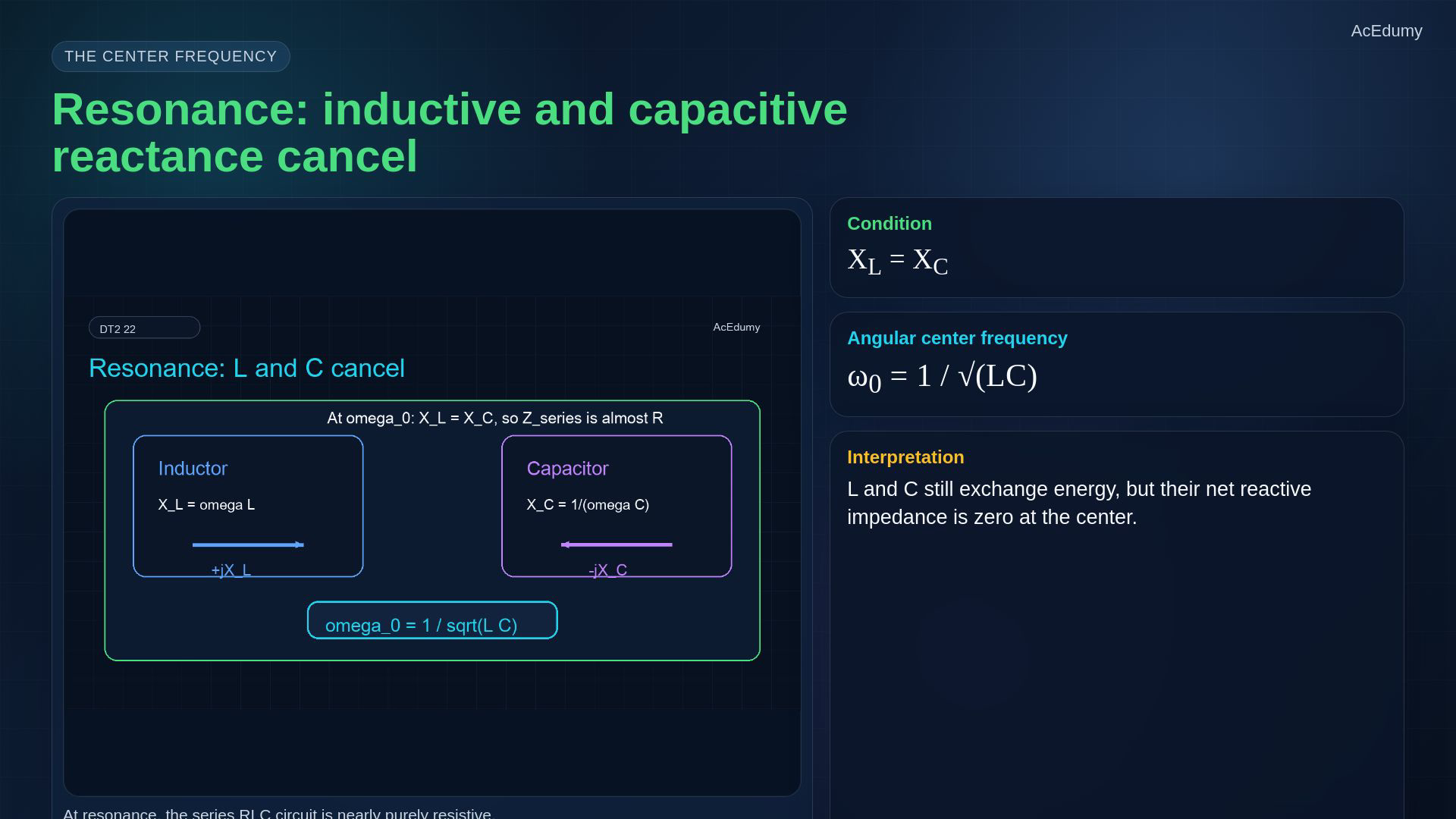
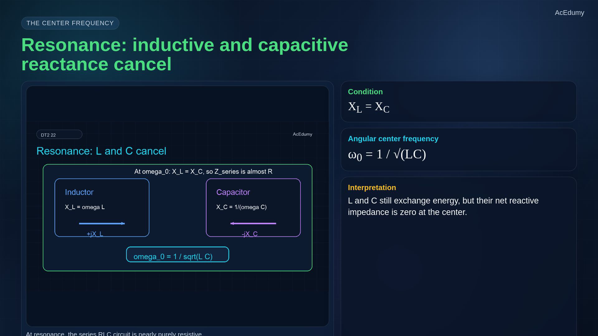
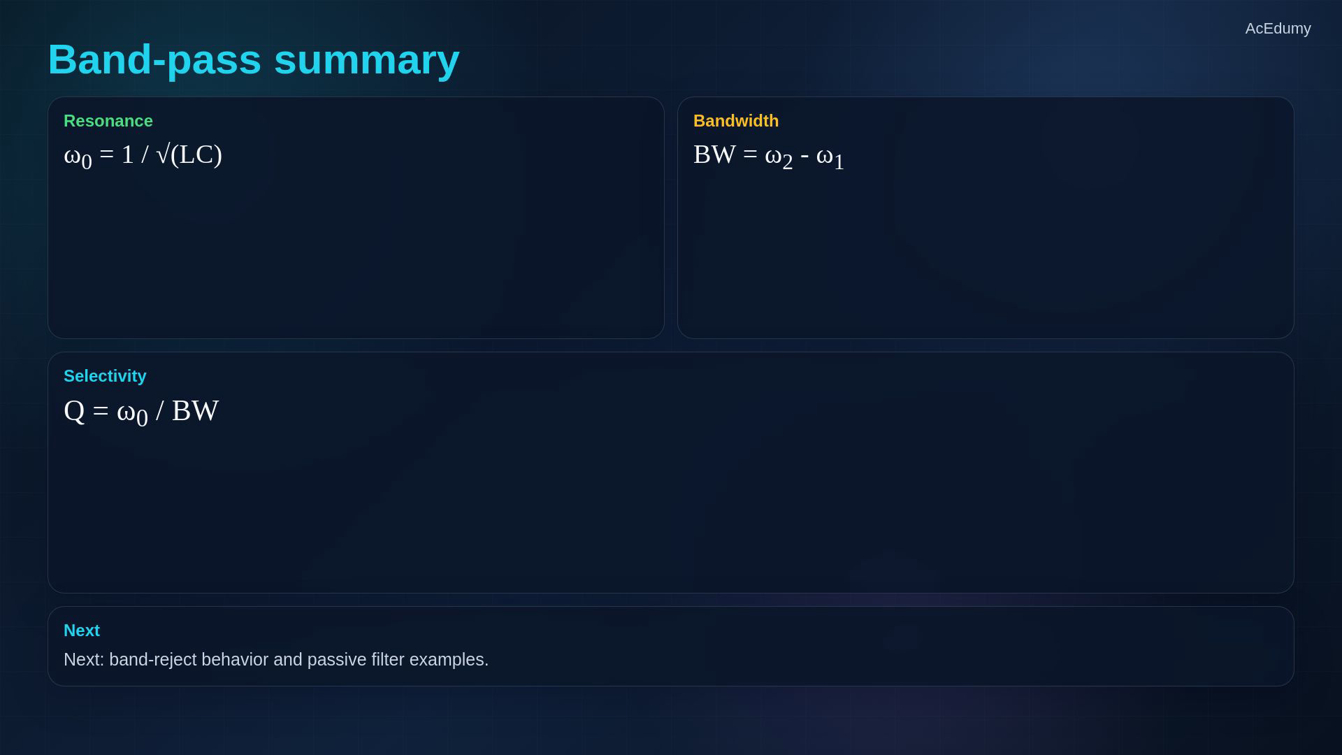
Resonance happens when the inductive reactance and capacitive reactance have equal magnitude. In formulas, omega naught equals one over square root of L C. At that frequency, X L and X C cancel in the series impedance, so the circuit looks almost purely resistive and the output across R peaks.
5. Read the normalized peak and falloff
The Q curves illustrate relative shape and equal peak height. Read their axes qualitatively; use the notebook formulas for exact cutoff values. Resonance and summary cards are reused for roles whose original plot or circuit reference is unsuitable.
The resistor response rises to resonance and then falls.
Normalized resonant voltage transfer:
$\displaystyle H\left(j\omega _{0}\right) = 1$
Read the falloff as well as the peak.
Narration transcript
On the magnitude plot, the band-pass curve rises from low frequency, peaks near the resonant frequency, then falls again. The peak is not magic amplification in a passive circuit; it is a voltage division result caused by the impedance becoming most favorable at resonance. The important reading is not only the peak, but also how quickly the response falls away on both sides.
6. Keep bandwidth units consistent
The Q curves illustrate relative shape and equal peak height. Read their axes qualitatively; use the notebook formulas for exact cutoff values. Resonance and summary cards are reused for roles whose original plot or circuit reference is unsuitable.
Use the lower and upper half-power frequencies.
Relative cutoff magnitude:
$\displaystyle |H\left(j\omega _{1}\right)| = |H\left(j\omega _{2}\right)| = 1/\sqrt{2}$
Angular bandwidth:
$\displaystyle B_{\omega } = \omega _{2} - \omega _{1}$
Hertz bandwidth:
$\displaystyle B_{f} = f_{2} - f_{1}$
Narration transcript
The minus-three-decibel frequencies are called omega one and omega two. They are the points where the magnitude has fallen to one over square root of two of the peak value. The angular bandwidth is omega two minus omega one. In hertz, the bandwidth is f two minus f one.
7. Check selectivity without assuming a taller peak
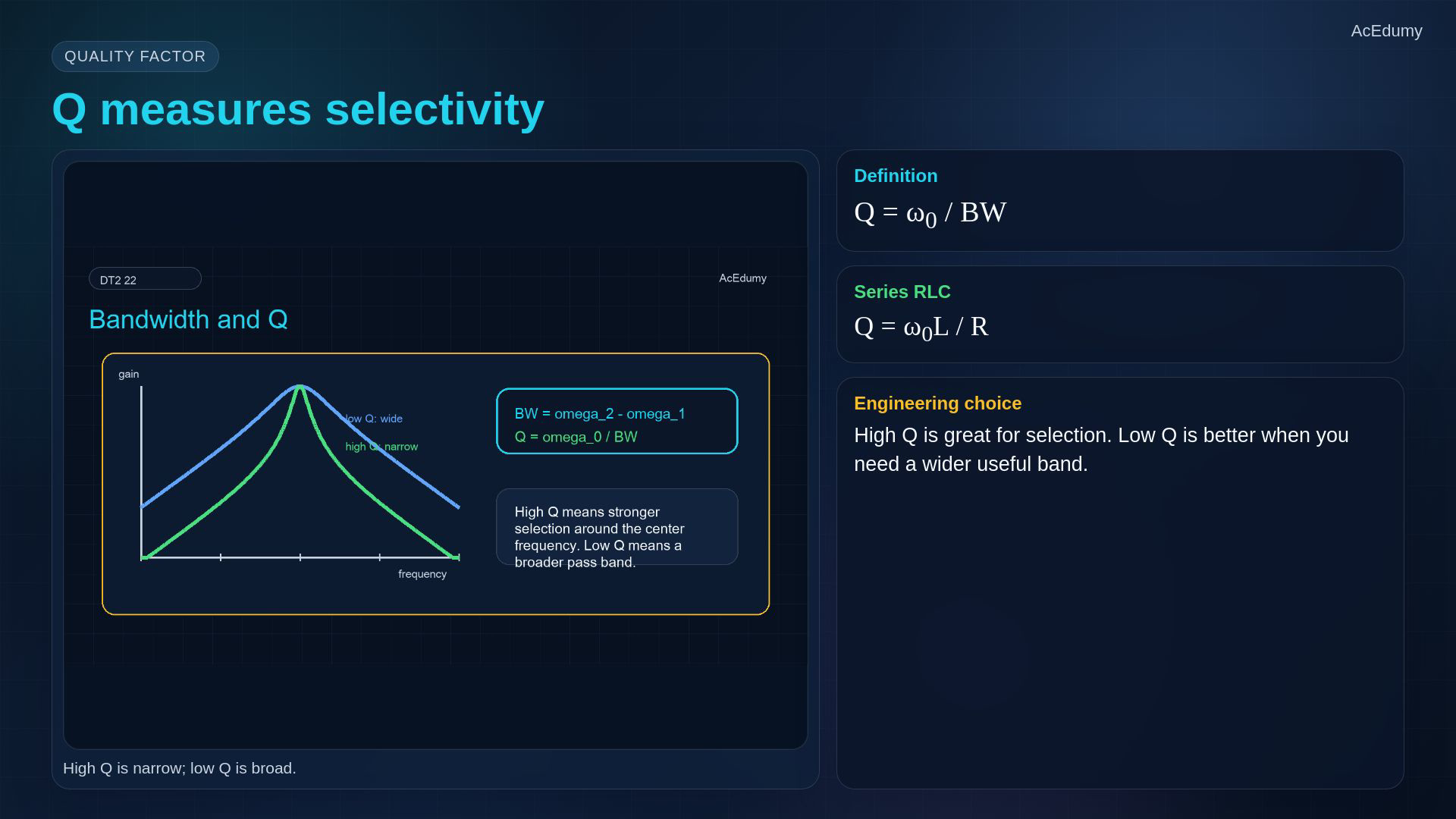
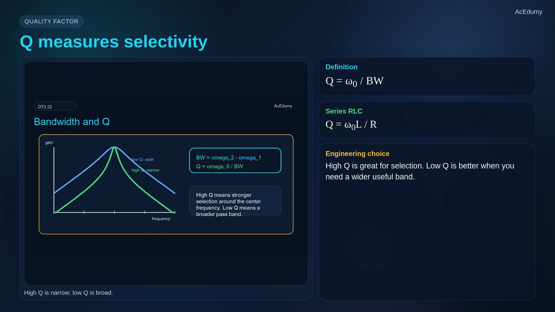
The Q curves illustrate relative shape and equal peak height. Read their axes qualitatively; use the notebook formulas for exact cutoff values. Resonance and summary cards are reused for roles whose original plot or circuit reference is unsuitable.
Q compares center frequency with bandwidth.
Dimensionless selectivity:
$\displaystyle Q =\frac{ \omega _{0}}{B_{\omega } }=\frac{ f_{0}}{B_{f}}$
A tall, narrow appearance means a sharper shape; the normalized peak stays one.
Lower Q gives a broader pass band.
For this ideal series circuit:
$\displaystyle Q =\frac{ \omega _{0} L}{R}$
Narration transcript
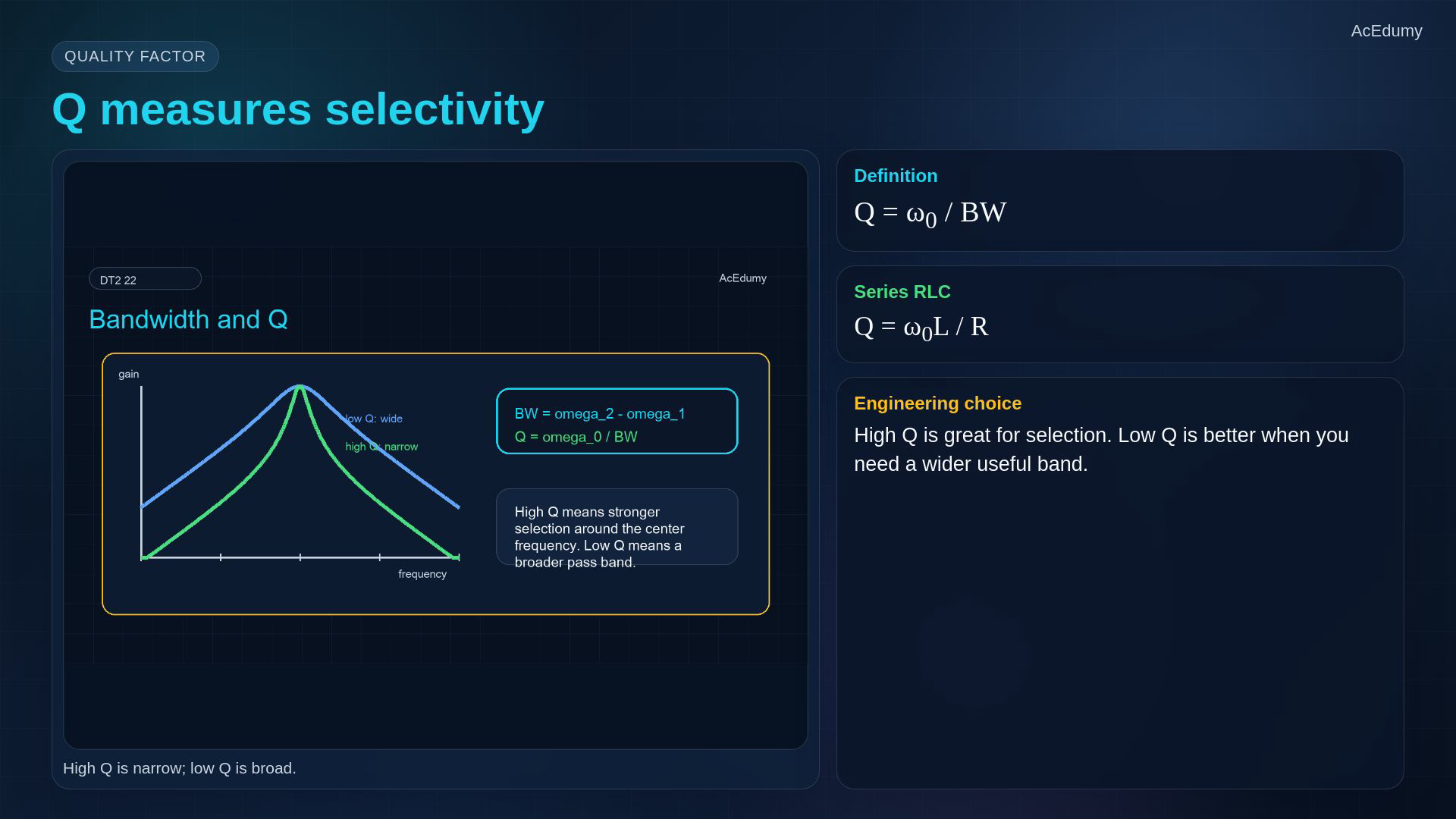
The quality factor, Q, compares the center frequency to the bandwidth. Q equals omega naught divided by bandwidth, or f naught divided by bandwidth in hertz. High Q means a tall, narrow, selective response. Low Q means a broad response. In a series RLC band-pass, Q also equals omega naught L over R.
8. Relate output phase to series impedance
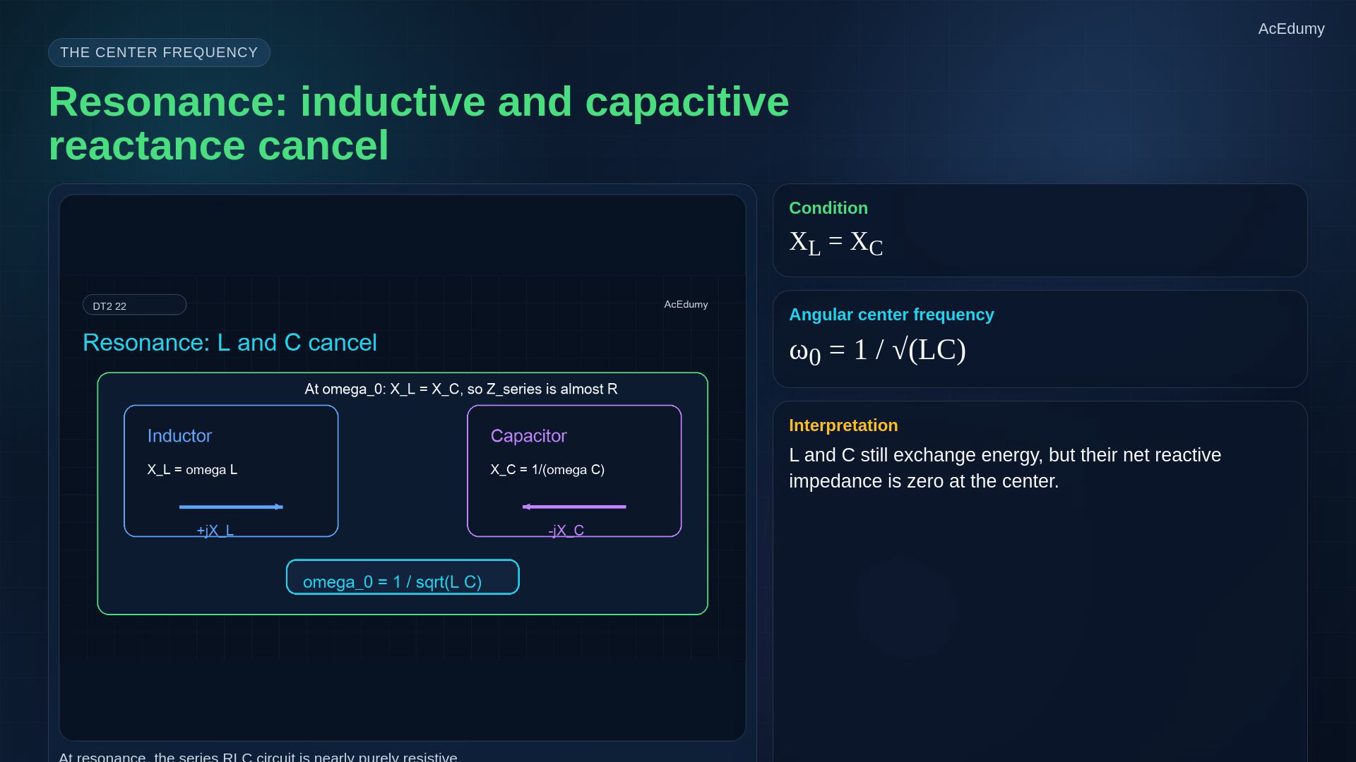
The Q curves illustrate relative shape and equal peak height. Read their axes qualitatively; use the notebook formulas for exact cutoff values. Resonance and summary cards are reused for roles whose original plot or circuit reference is unsuitable.
Relate phase to the reactive impedance.
Below resonance the net series reactance is capacitive.
Above resonance the net series reactance is inductive.
At resonance the resistor voltage is in phase with the source.
L and C still exchange energy while their net reactance vanishes.
Narration transcript
Phase gives another view of the same physics. Below resonance, the circuit behaves more capacitive. Above resonance, it behaves more inductive. At resonance, the reactive terms cancel and the resistor voltage is in phase with the source. Energy is still moving back and forth between L and C, but the net reactive impedance is zero at the center.
9. Calculate resonance, Q and bandwidth
The Q curves illustrate relative shape and equal peak height. Read their axes qualitatively; use the notebook formulas for exact cutoff values. Resonance and summary cards are reused for roles whose original plot or circuit reference is unsuitable.
Design example with ideal nominal components
Ten millihenries and one hundred nanofarads give about 5.03 kHz.
With one hundred ohms, Q is about 3.16 and bandwidth about 1.59 kHz.
At fixed L and C:
$\displaystyle B_{\omega } =\frac{ R}{L}$
Narration transcript
A quick design example. If L is ten millihenries and C is one hundred nanofarads, then f naught is about five point zero three kilohertz. If R is one hundred ohms, then Q is about three point one six, and the bandwidth is about one point five nine kilohertz. Changing R is the easiest way to widen or narrow the pass band.
10. Check loading, loss and bandwidth assumptions
The Q curves illustrate relative shape and equal peak height. Read their axes qualitatively; use the notebook formulas for exact cutoff values. Resonance and summary cards are reused for roles whose original plot or circuit reference is unsuitable.
Three checks before applying the ideal result
Center frequency and bandwidth describe different properties.
Higher Q is not always the better design choice.
Match the selectivity to the wanted frequency band.
Component loss and finite loading can change the effective response.
Narration transcript
Three traps. First, resonance frequency and bandwidth are different ideas; do not mix them. Second, Q is not automatically good or bad. High Q is useful for selection, but bad if you need a flat wide band. Third, real coils have resistance, real capacitors have loss, and any load connected to the filter changes the effective Q.
11. Summarize the series RLC response
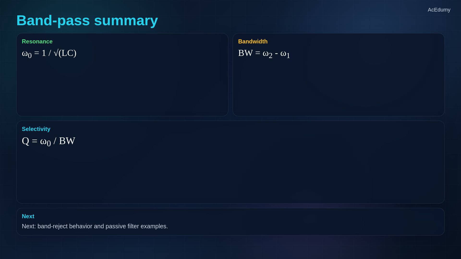
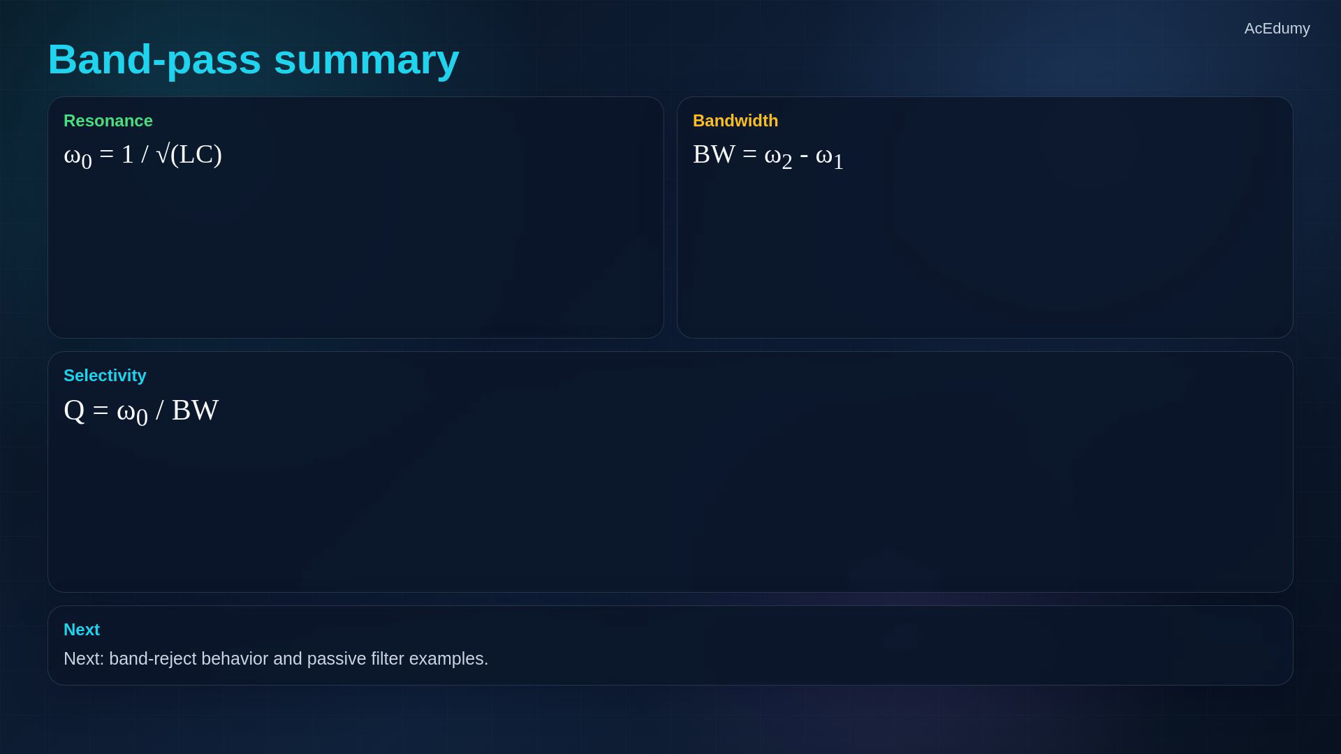
The Q curves illustrate relative shape and equal peak height. Read their axes qualitatively; use the notebook formulas for exact cutoff values. Resonance and summary cards are reused for roles whose original plot or circuit reference is unsuitable.
Series RLC band-pass recap
The resistor output keeps a middle frequency band.
Angular center frequency:
$\displaystyle \omega _{0} = 1/\sqrt{L C}$
Selectivity with angular bandwidth:
$\displaystyle Q =\frac{ \omega _{0}}{B_{\omega }}$
Next compare band-reject and other passive filter responses.
Narration transcript
Summary. A band-pass filter keeps a middle frequency band. In a series RLC band-pass, resonance occurs at one over square root L C. The minus-three-decibel points define bandwidth, and Q equals center frequency divided by bandwidth. Next we use the same ideas to build a band-reject filter and compare passive filter examples.