#18 The Biot-Savart law, right-hand rule, line/surface/volume current distributions, and the magnetic field of a straight conductor

Below are all the lines written in the notebook together with the full narration transcript.

1. 1. Move from electrostatics to magnetostatics

   

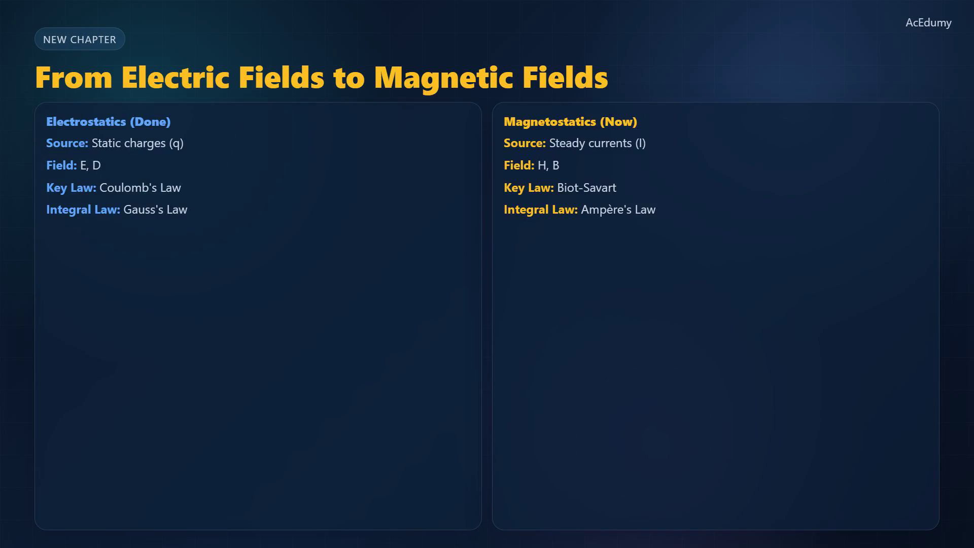
   So far, everything we've studied has been about electric fields created by static charges.

   Coulomb's law, Gauss's law, electric potential — all of that was electrostatics.

   Now we enter a brand new chapter: magnetostatics.

   Here, the source is not a stationary charge but a steady current.

   And the first question is: what magnetic field does a current produce?

   The answer is the Biot-Savart law.

   Narration transcript

   So far, everything we've studied has been about electric fields created by static charges. Coulomb's law, Gauss's law, electric potential — all of that was electrostatics. Now we enter a brand new chapter: magnetostatics. Here, the source is not a stationary charge but a steady current. And the first question is: what magnetic field does a current produce? The answer is the Biot-Savart law.

2. 2. Build the Biot-Savart relation

   

   Consider a thin wire carrying a steady current I.

   Take a tiny piece of this wire — we call it dl.

   This small element creates a magnetic field dH at some point P, located a distance R away.

   dH = I dl × â_R/(4πR²).

   Let's break this apart.

   The magnitude is proportional to the current I and the element length dl.

   It falls off as 1 over R² — just like Coulomb's law.

   And the direction comes from the cross product: dH is perpendicular to both the current element and the line from the element to point P.

   Narration transcript

   Consider a thin wire carrying a steady current I. Take a tiny piece of this wire — we call it d l. This small element creates a magnetic field d H at some point P, located a distance R away. Biot and Savart discovered that d H equals I d l cross a-hat-R, divided by 4 pi R squared. Let's break this apart. The magnitude is proportional to the current I and the element length d l. It falls off as 1 over R squared — just like Coulomb's law. And the direction comes from the cross product: d H is perpendicular to both the current element and the line from the element to point P.

3. 3. Determine field direction

   

   The direction of H follows the right-hand rule.

   Point your right thumb along the current.

   Your fingers curl around the wire, and that curl direction is the direction of H.

   For a current going into the page, H circulates clockwise.

   For a current coming out of the page, it goes counterclockwise.

   We mark these with a cross for into the page, and a dot for out of the page.

   Narration transcript

   The direction of H follows the right-hand rule. Point your right thumb along the current. Your fingers curl around the wire, and that curl direction is the direction of H. For a current going into the page, H circulates clockwise. For a current coming out of the page, it goes counterclockwise. We mark these with a cross for into the page, and a dot for out of the page.

4. 4. Compare three current distributions

   

   Biot-Savart works for any current distribution, not just thin wires.

   Line current: H = ∫ I dl × â_R/(4πR²).

   Surface current: H = ∫ K dS × â_R/(4πR²), with K in A/m.

   Volume current: H = ∫ J dv × â_R/(4πR²), with J in A/m².

   Equivalent current elements: I dl = K dS = J dv.

   Narration transcript

   Biot-Savart works for any current distribution, not just thin wires. For a line current, we integrate I d l along the path. For a surface current with density K amperes per meter, we integrate K d S over the surface. For a volume current with density J amperes per square meter, we integrate J d v over the volume. The link between them is simple: I d l equals K d S equals J d v.

5. 5. Evaluate the straight-wire integral

   

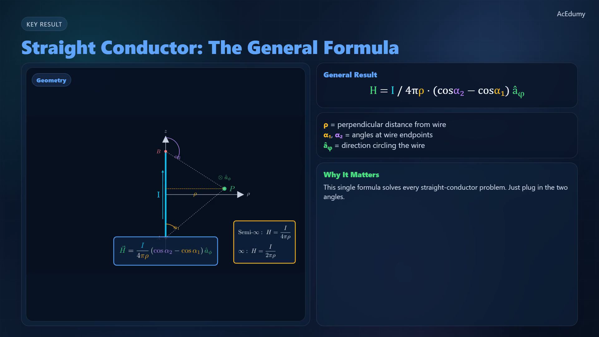
   Now let's apply Biot-Savart to the most common case: a straight wire carrying current I.

   Place the conductor along the z-axis, and pick a point P at a perpendicular distance ρ from the wire.

   The wire extends between two endpoints.

   We define α₁ as the angle at the lower end and α₂ at the upper end, both measured from the wire axis.

   The source audio/figure states H = I/(4πρ)(cos α₂ − cos α₁); with the endpoint-angle definitions drawn in the figure, the derivation requires H = I/(4πρ)(cos α₁ − cos α₂) â_φ.

   The direction is along â_φ — circling the wire.

   This single formula covers every straight-conductor problem.

   Narration transcript

   Now let's apply Biot-Savart to the most common case: a straight wire carrying current I. Place the conductor along the z-axis, and pick a point P at a perpendicular distance rho from the wire. The wire extends between two endpoints. We define alpha 1 as the angle at the lower end and alpha 2 at the upper end, both measured from the wire axis. After integrating the Biot-Savart law along the wire, we get: H equals I over 4 pi rho, times the quantity cosine alpha 2 minus cosine alpha 1. The direction is along a-hat-phi — circling the wire. This single formula covers every straight-conductor problem.

6. 6. Analyze semi-infinite and infinite wires

   

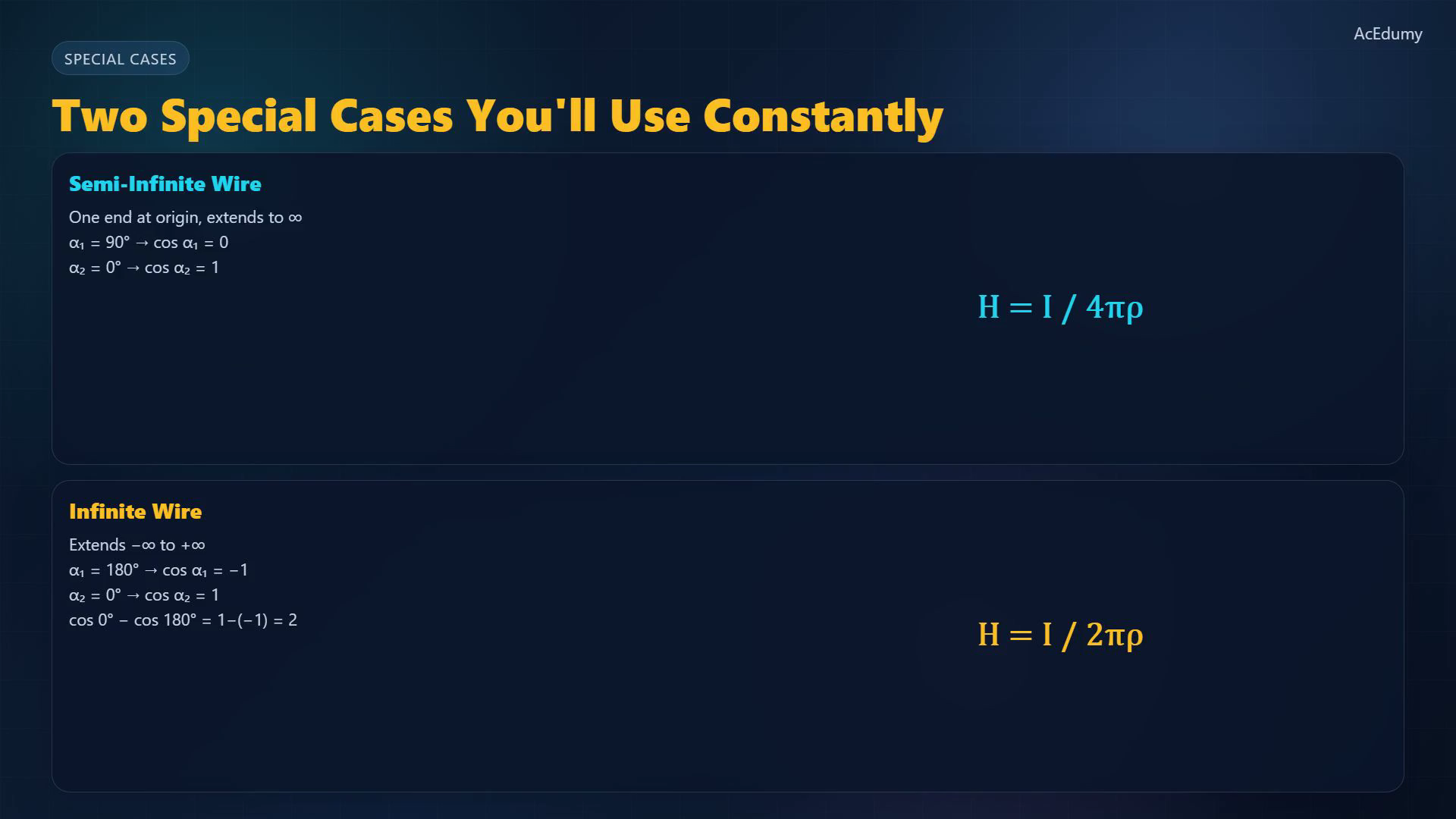
   Two special cases come up constantly.

   First, a semi-infinite wire: one end at the origin, extending to infinity along z.

   With the endpoint-angle convention drawn in the figure, a semi-infinite wire has α₁ = 90°, α₂ = 180°, and H = I/(4πρ).

   Second, and most important, an infinite wire stretching from minus infinity to plus infinity.

   With the endpoint-angle convention drawn in the figure, an infinite wire has α₁ = 0° and α₂ = 180°.

   The cosines give us 1 minus negative 1, which is 2.

   Thus H = I/(2πρ).

   This is probably the single most important result in magnetostatics.

   Narration transcript

   Two special cases come up constantly. First, a semi-infinite wire: one end at the origin, extending to infinity along z. Here, alpha 1 is 90 degrees and alpha 2 is 0, so the formula gives H equals I over 4 pi rho. Second, and most important, an infinite wire stretching from minus infinity to plus infinity. Now alpha 1 is 180 degrees and alpha 2 is 0. The cosines give us 1 minus negative 1, which is 2. So H equals I over 2 pi rho. This is probably the single most important result in magnetostatics.

7. 7. Review the Biot-Savart results

   

   To wrap up: the Biot-Savart law tells us the magnetic field from any current distribution.

   For straight conductors, it boils down to a formula with two angles.

   For an infinite wire, H = I/(2πρ).

   In the next video, we'll apply these formulas to solve example problems step by step.

   Narration transcript

   To wrap up: the Biot-Savart law tells us the magnetic field from any current distribution. For straight conductors, it boils down to a formula with two angles. And for an infinite wire, the result simplifies to I over 2 pi rho. In the next video, we'll apply these formulas to solve example problems step by step.

Source video: Electromagnetic Theory (v2) #18 The Biot-Savart Law (4:12)