Electronics 1 · Electronics Basics
#20 BJT graphical DC analysis — load line and Q-point
Read beta from the output characteristics, solve the base loop, and locate the Q-point algebraically and graphically with the DC load line.
Question
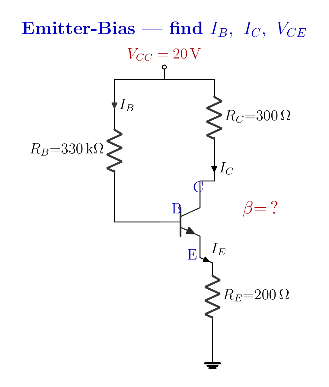
An emitter-resistor BJT circuit has V_CC=20 V, R_B=330 kΩ, R_C=300 Ω, and R_E=200 Ω; beta is not supplied. Determine beta from the output curves, calculate I_B, I_C, and V_CE, then draw the DC load line and locate the Q-point.
Written solution and narration transcript(shows the full solution)
Below are all the lines written in the notebook together with the full narration transcript.
1. Two views, one operating point
Beta is not supplied; read it from the output curves before solving I_B, I_C, and V_CE. Given: 20 V, 330 kΩ, 300 Ω, 200 Ωβ is missing → read it from the graphDevice constraint: output curvesCircuit constraint: DC load lineTheir intersection is the operating pointNarration transcript
Welcome back. We have solved a whole family of bias circuits with algebra: write the loops, push the numbers through. Today we add a second pair of eyes, the graph. And we start with a twist. Look at this transistor: its current gain, beta, is not given to us. In every problem so far beta was handed over. Here it is missing. But it is not really missing, it is hiding in plain sight, printed on the transistor's own characteristic curves. Our job is the usual three numbers: the base current, the collector current, and the collector-emitter voltage. To get them we will meet two characters. The first is the device: the transistor's output curves, which show everything the transistor itself can do. The second is the circuit: a single straight line, the load line, that captures everything the resistors will allow. The operating point, the one place the transistor actually settles, is wherever those two agree. Picture two lines on a chart crossing once. The device says, I can be anywhere along my curve; the circuit says, I can be anywhere along my line; and only their crossing satisfies both at once. Let us find it.
2. Read beta from the curves
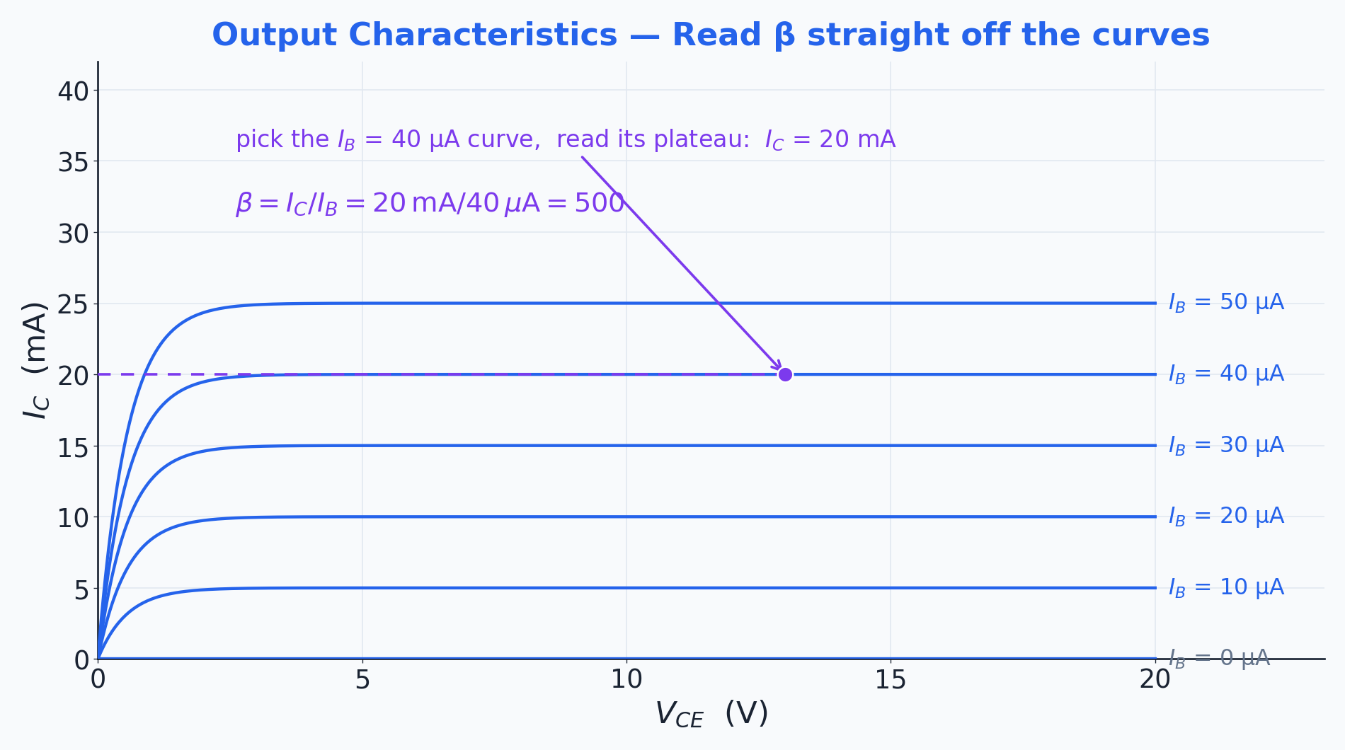
In the flat active region, the ratio I_C/I_B gives the current gain. Choose the IB = 40 µA curveActive-region plateau: IC ≈ 20 mAβ = 20 mA / 40 µANarration transcript
Here are the transistor's output characteristics. Each curve is the collector current as the collector-emitter voltage changes, and there is one curve for each base current: ten microamps, twenty, on up to fifty. Notice the shape. Each one shoots up fast, then flattens into a plateau and stays there. That flat plateau is the active region, where the transistor acts like a current source set by the base. And here is the gift. On the flat part, the collector current is simply beta times the base current. So to find beta we do not need a datasheet, we read it straight off the graph. Take the forty-microamp curve. Follow it across to its plateau and read the collector current: twenty milliamps. Beta is just the ratio, twenty milliamps divided by forty microamps. Twenty over forty is one half, and milliamps over microamps is a thousand, so beta is five hundred. The curves handed us the gain. Now we can solve the circuit.
3. Base current
Beta is not supplied; read it from the output curves before solving I_B, I_C, and V_CE. Base loopNarration transcript
Now the algebra, starting with the base side. Walk the base loop: from the supply, down through the base resistor, across the base-emitter junction, and down through the emitter resistor to ground. In words: twenty volts, minus the base current through three hundred thirty k, minus the usual 0.7 across the junction, minus the emitter drop. The one subtlety is the emitter. The current there is not the base current, it is beta-plus-one times bigger, the base current plus the collector current it controls. So the emitter resistor, felt from the base, acts like five hundred and one times two hundred ohms. Add that to the base resistor: three hundred thirty k, plus five hundred one times two hundred, which is about a hundred k more. Together, roughly four hundred thirty k. The driving voltage is twenty minus 0.7, which is 19.3 volts. So the base current is 19.3 volts over four hundred thirty k, about forty-five microamps. A tiny base current, exactly what we expect for a base fed through such a large resistor.
4. Algebraic operating point
Beta is not supplied; read it from the output curves before solving I_B, I_C, and V_CE. IC = βIB ≈ 22.5 mAVRC ≈ 300 Ω·22.5 mA = 6.75 VVRE ≈ 200 Ω·22.5 mA = 4.50 VNarration transcript
With the base current and beta in hand, the collector current is immediate: collector current equals beta times base current, five hundred times forty-five microamps, which is twenty-two point five milliamps. Now the last unknown, the collector-emitter voltage. Walk the output loop this time: from the supply, down through the collector resistor, across the transistor, and down through the emitter resistor. The collector resistor drops three hundred ohms times twenty-two point five milliamps, which is 6.75 volts. The emitter resistor drops two hundred ohms times the emitter current, and the emitter current is essentially the collector current, about twenty-two and a half milliamps, so that is 4.5 volts. The collector-emitter voltage is what is left of the twenty: twenty minus 6.75 minus 4.5, which is eight point seven four volts. There it is, the algebra's answer for the operating point: twenty-two point five milliamps at eight point seven four volts.
5. The DC load line
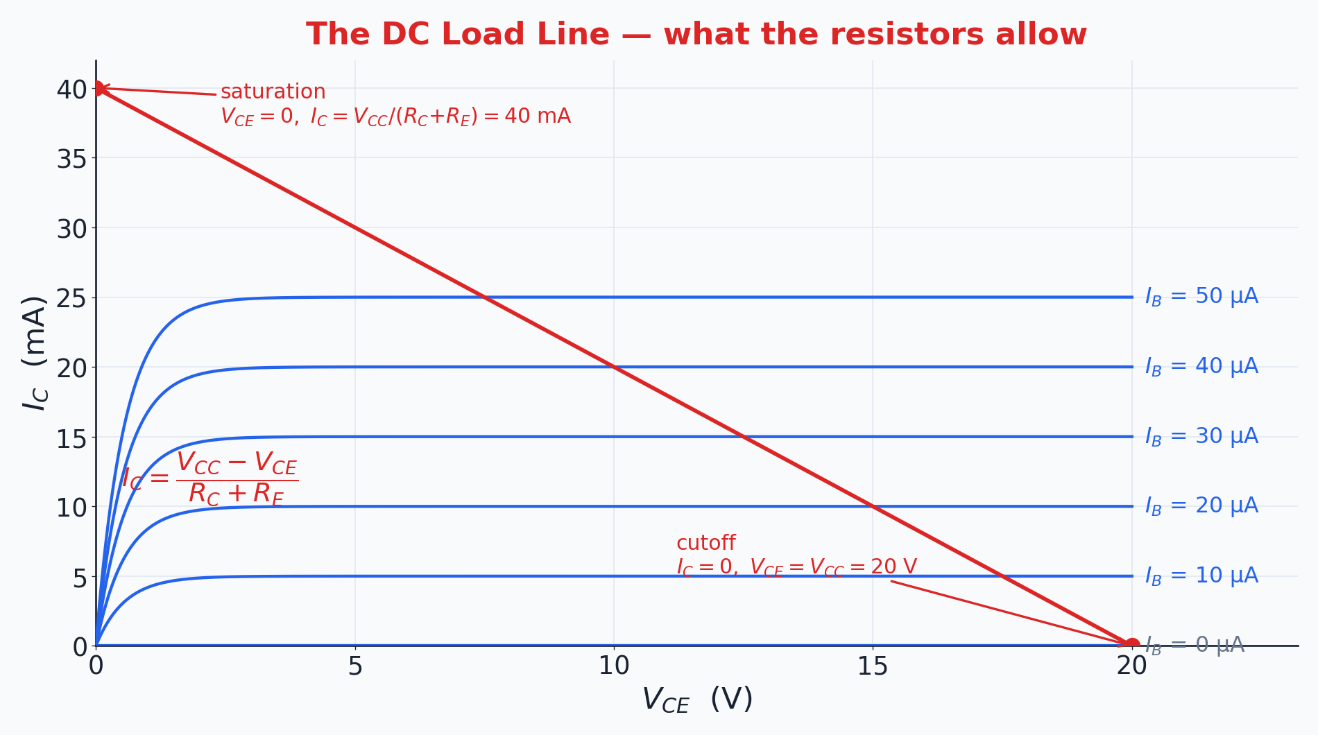
The load line joins (20 V, 0 mA) and (0 V, 40 mA). Cutoff:Other endpoint: VCE=0 → IC=40 mA(20 V, 0 mA) ↔ (0 V, 40 mA)Join the endpoints → load lineNarration transcript
Now let us see that same answer appear on the graph, through the load line. Go back to the output loop, but this time solve it for the collector current as a function of the collector-emitter voltage. Rearranged, the collector current is the supply minus the collector-emitter voltage, all over the sum of the two resistors, three hundred plus two hundred, which is five hundred ohms. That is the equation of a straight line, and a line needs just two points. First, imagine the transistor fully off, cutoff. No collector current, so no drop across the resistors, and the whole twenty volts appears across the transistor. That is the point twenty volts, zero milliamps, on the right. Second, imagine it fully on, saturation. The collector-emitter voltage collapses to zero, and the current is just the supply over the two resistors, twenty over five hundred, which is forty milliamps. That is the point zero volts, forty milliamps, up top. Connect those two points and you have drawn the load line: every operating point the resistors will permit, all on one straight stroke.
6. The Q-point
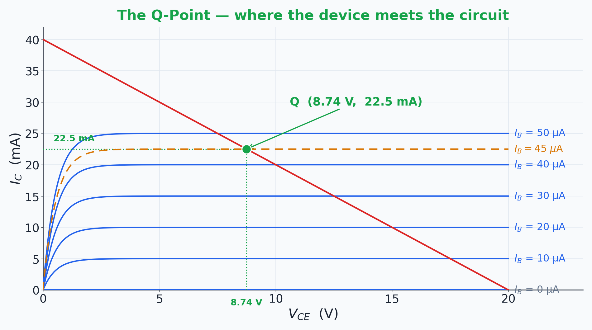
The operating point is approximately V_CE=8.74 V and I_C=22.5 mA. Use the IB ≈ 45 µA characteristicThe point must lie on both curve and load lineIntersection = Q-pointQ ≈ (VCE=8.74 V, IC=22.5 mA)Graph and algebra agreeNarration transcript
Now bring the two characters together. The device gave us the family of curves; the circuit gave us the load line. Lay the line right on top of the curves. The transistor must live on its curve, and it must also live on the load line, so it sits exactly where they cross. Which curve? The one for our base current, forty-five microamps, sitting between the forty and the fifty. Follow the load line until it meets that curve, and drop down to the axes. You land at eight point seven four volts and twenty-two point five milliamps, the very same numbers the algebra gave us. That crossing point has a name: the Q-point, the quiescent operating point. It is the handshake between the device and the circuit, the single state where the transistor obeys its own physics and the circuit's voltage law at the same time. Two methods, one point.
7. Method summary
The operating point is approximately V_CE=8.74 V and I_C=22.5 mA. 1) Read β from the curves2) Solve IB from the base loop3) Use βIB for IC; KVL for VCE4) Draw the load line from two endpoints5) Read the Q-point at the intersectionβ≈500; IB≈45 µA; IC≈22.5 mA; VCE≈8.74 VNarration transcript
Let us gather it up. We were handed a transistor with no beta, and we read it straight off the output curves: twenty milliamps over forty microamps gives five hundred. Then the base loop gave a base current of forty-five microamps; beta times that is a collector current of twenty-two and a half milliamps; and the output loop left eight point seven four volts across the transistor. Finally we drew the load line, cutoff at twenty volts, saturation at forty milliamps, and watched the Q-point appear exactly where the line crosses the forty-five-microamp curve. The headline to carry: the operating point is where the device meets the circuit. The curves are the transistor's personality; the load line is the circuit's demand; the Q-point is the one place both are honored. And with that, our DC tour of the bipolar transistor is complete. Next, we meet a different breed entirely, the field-effect transistor, where a voltage, not a current, takes command. See you there.
Source video: Electronics Basics #20 | BJT Graphical DC Analysis: Load Line and Q-Point (8:18)