Control Theory · Bode Phase Plot — Lecture 5, Part 3

#46 Numerator/denominator phase signs, LHP and RHP factors, the two-decade phase approximation, unwrapped phase, and scoped phase-margin interpretation

Add factor phases with the correct signs, verify the two-decade approximation with exact atan2 calculations, and interpret phase margin together with Nyquist conditions.

Question

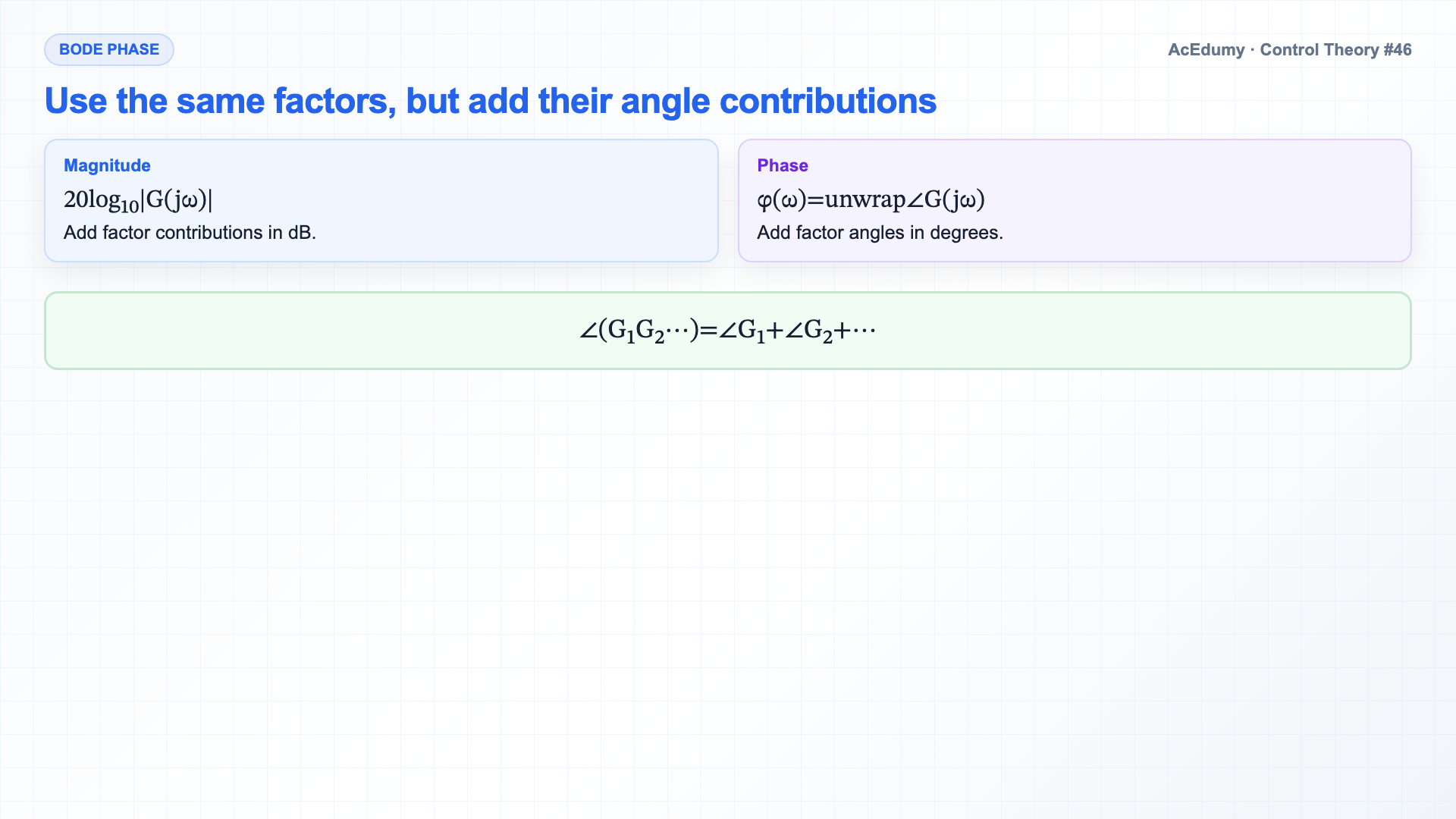
English solution frame showing Bode-phase atoms, the decade approximation, unwrapped phase, and the scope of phase-margin interpretation. — For G(s)=10/[s(s+1)(s+10)], exact phase is −90°−atan(ω)−atan(ω/10), while the asymptote moves from −90° to −270°.

Construct a Bode phase plot from elementary factor contributions. Compute the exact and asymptotic phase of G(s)=10/[s(s+1)(s+10)], and explain RHP-zero normalization, phase unwrapping, and the conditions required for phase-margin interpretation.

Written solution and narration transcript(shows the full solution)

Below are all the lines written in the notebook together with the full narration transcript.

1. Establish the Bode-phase sum rule
For G(s)=10/[s(s+1)(s+10)], exact phase is −90°−atan(ω)−atan(ω/10), while the asymptote moves from −90° to −270°.
Last lecture we drew the Bode magnitude — factor decomposition, sum of dB asymptotes, three lines and you are done.
Today, the second half of the Bode plot.
The phase.
Same factoring trick.
Different rules.
Same speed.
Narration transcript
Last lecture we drew the Bode magnitude — factor decomposition, sum of dB asymptotes, three lines and you are done. Today, the second half of the Bode plot. The phase. Same factoring trick. Different rules. Same speed.
2. Explain numerator and denominator phase signs
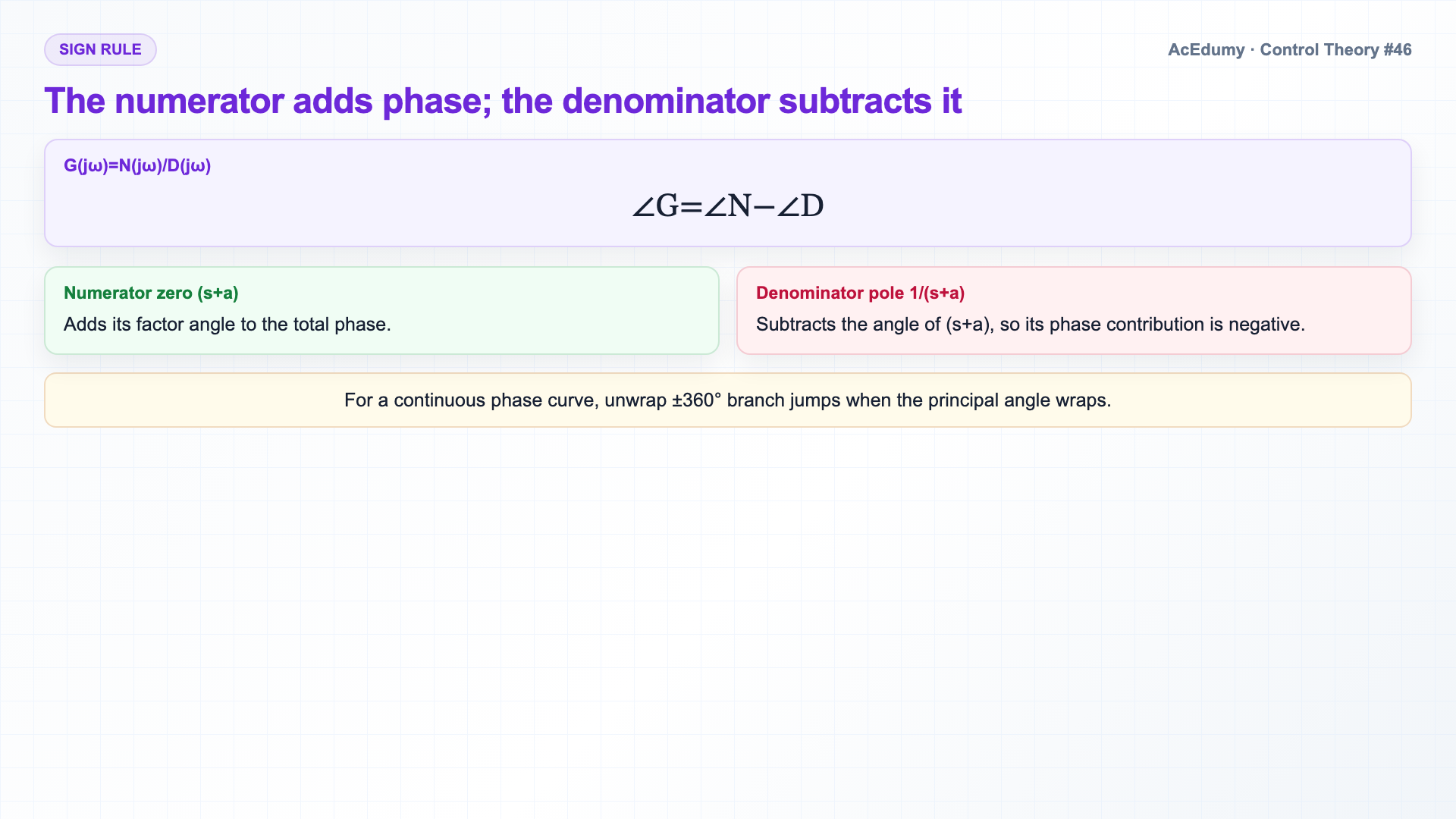
For G(s)=10/[s(s+1)(s+10)], exact phase is −90°−atan(ω)−atan(ω/10), while the asymptote moves from −90° to −270°.
Why phases add.
The angle of a product equals the sum of the angles.
∠(GH)=∠G+∠H (mod 360°); unwrap branch jumps when a continuous Bode phase is required.
So when we factor a transfer function into atoms, the total phase is the sum of each atom's phase contribution.
$\displaystyle ∠\left(\frac{N}{D}\right)=∠N-∠D.$
A numerator zero (s+a) adds its factor angle; a denominator pole (s+a) subtracts it, so 1/(s+a) has a negative phase contribution.
Mirror images.
Just like with magnitude, we get a sum of asymptotes — only this time the asymptotes live on a phase axis, marked in degrees.
Narration transcript
Why phases add. The angle of a product equals the sum of the angles. Angle of G times H is angle of G plus angle of H. So when we factor a transfer function into atoms, the total phase is the sum of each atom's phase contribution. And division flips the sign — angle of one over G is minus angle of G. So a denominator factor like one over s plus a contributes minus its phase, while a numerator factor like s plus a contributes plus its phase. Mirror images. Just like with magnitude, we get a sum of asymptotes — only this time the asymptotes live on a phase axis, marked in degrees.
3. Separate the LHP and RHP phase-atom rules
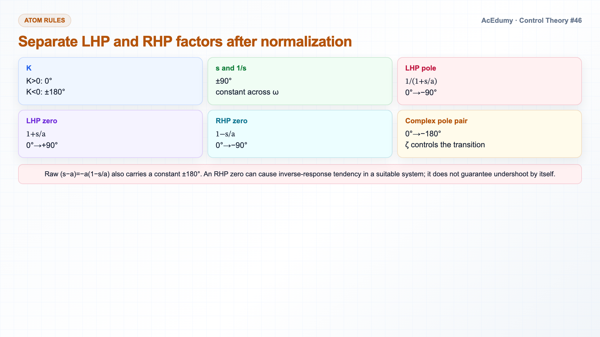
For G(s)=10/[s(s+1)(s+10)], exact phase is −90°−atan(ω)−atan(ω/10), while the asymptote moves from −90° to −270°.
Phase rules per atom.
Constant K≠0.
K>0 has phase 0°; K<0 has +180° or −180° depending on the selected branch.
A flat horizontal line.
Integrator one over s.
Phase is constant minus ninety degrees, at every frequency.
Differentiator s — plus ninety degrees.
An n-fold integrator one over s to the n contributes minus ninety n degrees.
Pure constant offsets.
For a>0, the normalized simple LHP pole is 1/(1+s/a).
Its exact phase is −atan(ω/a), approaching 0° as ω→0 and −90° as ω→∞.
The transition is smooth, centered at the corner.
Simple zero s plus a.
Mirror image.
The normalized LHP zero 1+s/a has exact phase +atan(ω/a), with limits 0° and +90°.
For a>0, the normalized RHP zero is 1−s/a; raw (s−a)=−a(1−s/a) also carries a constant ±180°.
The factor 1−s/a shares magnitude with the LHP zero but has phase −atan(ω/a), approaching −90° from 0°.
This non-minimum-phase signature can produce inverse-response tendency in a suitable system, but an RHP zero alone does not guarantee undershoot.
We will revisit this in compensator design.
Complex conjugate pair.
Phase rotates twice as fast — zero below the natural frequency, minus one hundred eighty above, with a steep transition controlled by the damping ratio.
Narration transcript
Phase rules per atom. Constant K. Phase is zero degrees if K is positive, plus or minus one hundred eighty degrees if K is negative. A flat horizontal line. Integrator one over s. Phase is constant minus ninety degrees, at every frequency. Differentiator s — plus ninety degrees. An n-fold integrator one over s to the n contributes minus ninety n degrees. Pure constant offsets. Simple pole one over s plus a. Phase is zero below the corner, minus ninety above the corner. The transition is smooth, centered at the corner. Simple zero s plus a. Mirror image. Zero below, plus ninety above. Right-half-plane zero, s minus a with positive a. Same magnitude behavior as a left-half-plane zero, but the phase goes minus ninety instead of plus ninety. This is the non-minimum phase signature — physically it produces undershoot in step response. We will revisit this in compensator design. Complex conjugate pair. Phase rotates twice as fast — zero below the natural frequency, minus one hundred eighty above, with a steep transition controlled by the damping ratio.
4. Construct the decade phase approximation for a simple factor
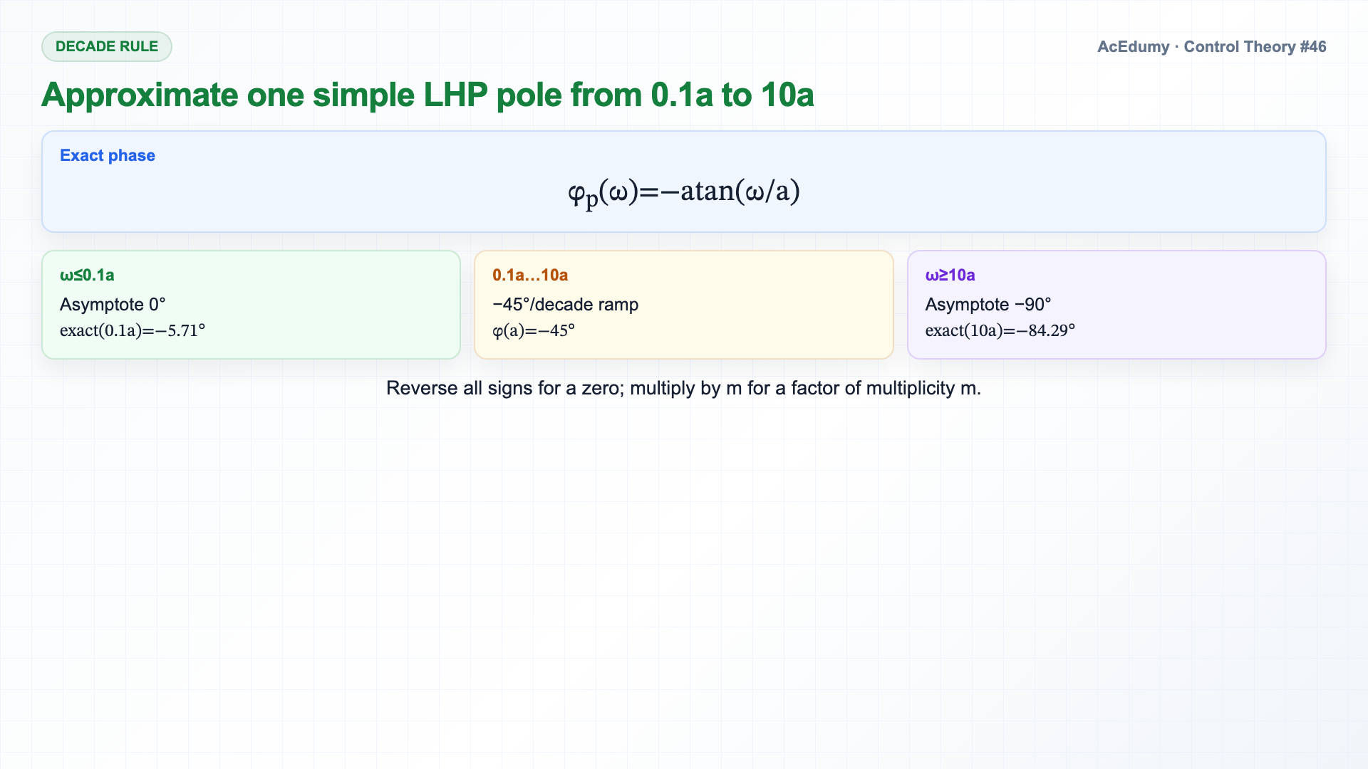
For G(s)=10/[s(s+1)(s+10)], exact phase is −90°−atan(ω)−atan(ω/10), while the asymptote moves from −90° to −270°.
The decade rule.
For a simple pole or zero with corner at omega equals a, the asymptotic phase transition can be drawn as three line segments.
First — flat asymptote at zero, holding for ω less than a divided by ten.
Second — a straight ramp from zero to plus or minus ninety degrees, between ω equals a divided by ten and ω equals ten times a.
The slope of this ramp is plus or minus forty-five degrees per decade.
Third — flat asymptote at the limit value, plus or minus ninety degrees, for ω greater than ten times a.
At the corner ω equals a exactly, the phase is plus or minus forty-five degrees — halfway through the ramp.
Useful checkpoints.
At ω=a/10, exact phase magnitude is atan(0.1)=5.71°, approximately 6.35% of the 90° limit.
At ω=10a, exact phase magnitude is atan(10)=84.29°, approximately 93.65% of the 90° limit.
Between, the ramp is the asymptote.
Narration transcript
The decade rule. For a simple pole or zero with corner at omega equals a, the asymptotic phase transition can be drawn as three line segments. First — flat asymptote at zero, holding for ω less than a divided by ten. Second — a straight ramp from zero to plus or minus ninety degrees, between ω equals a divided by ten and ω equals ten times a. The slope of this ramp is plus or minus forty-five degrees per decade. Third — flat asymptote at the limit value, plus or minus ninety degrees, for ω greater than ten times a. At the corner ω equals a exactly, the phase is plus or minus forty-five degrees — halfway through the ramp. Useful checkpoints. One decade below corner — phase is roughly five percent of the limit. One decade above — roughly ninety-five percent. Between, the ramp is the asymptote.
5. Solve the three-factor Bode-phase example
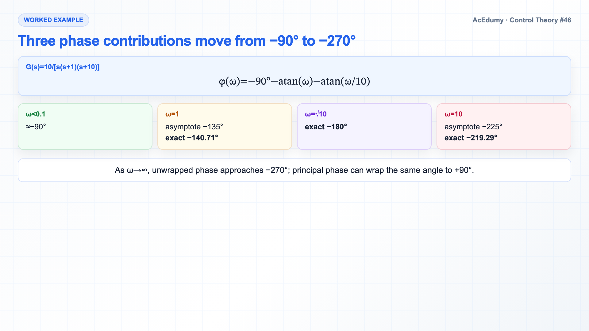
For G(s)=10/[s(s+1)(s+10)], exact phase is −90°−atan(ω)−atan(ω/10), while the asymptote moves from −90° to −270°.
Worked example.
Same transfer function from last lecture.
$\displaystyle G\left(s\right)=10/\left[s\left(s+1\right)\left(s+10\right)\right].$
Atoms.
Constant ten — positive, contributes zero degrees.
Integrator one over s — contributes minus ninety degrees, flat across all frequencies.
Two simple poles — corner at one and corner at ten, each contributing a transition from zero to minus ninety degrees, with the decade rule centered on its corner.
The exact unwrapped total phase is φ(ω)=−90°−atan(ω)−atan(ω/10).
Below ω equals zero point one, the phase is just the integrator contribution, minus ninety degrees.
Between zero point one and one, the first pole's transition starts.
At ω=1 the asymptote is −135°, while exact phase is −90°−45°−atan(0.1)=−140.71°.
Between one and ten, the first pole completes its drop and the second pole's transition begins.
Exact phase is −180° at ω=√10≈3.162; at ω=10 it is −219.29°, while the asymptote is −225°.
Above ω equals one hundred, both poles are deep in their asymptotic regime.
As ω→∞, unwrapped phase approaches −270°; principal phase can wrap the same angle to +90°.
Narration transcript
Worked example. Same transfer function from last lecture. G of s equals ten divided by s times s plus one times s plus ten. Atoms. Constant ten — positive, contributes zero degrees. Integrator one over s — contributes minus ninety degrees, flat across all frequencies. Two simple poles — corner at one and corner at ten, each contributing a transition from zero to minus ninety degrees, with the decade rule centered on its corner. Total. Below ω equals zero point one, the phase is just the integrator contribution, minus ninety degrees. Between zero point one and one, the first pole's transition starts. Phase ramps down from minus ninety toward minus one hundred thirty-five degrees by ω equals one. Between one and ten, the first pole completes its drop and the second pole's transition begins. The total phase reaches minus one hundred eighty around ω equals three or so, then continues toward minus two hundred twenty-five degrees by ω equals ten. Above ω equals one hundred, both poles are deep in their asymptotic regime. The phase settles at minus two hundred seventy degrees — minus ninety from the integrator, minus ninety from each pole, totaling minus two hundred seventy.
6. Compare exact and asymptotic phase
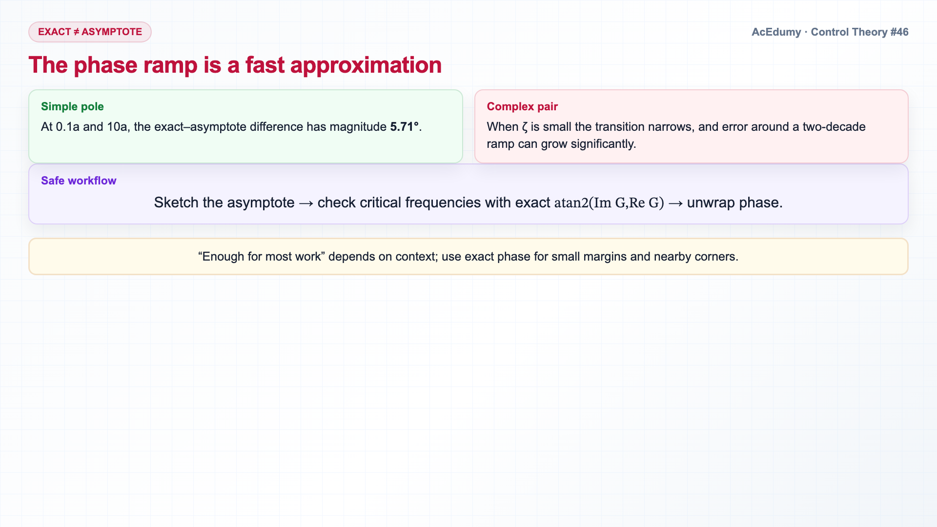
For G(s)=10/[s(s+1)(s+10)], exact phase is −90°−atan(ω)−atan(ω/10), while the asymptote moves from −90° to −270°.
How accurate is the asymptotic phase?
Quite accurate — but a bit looser than magnitude.
For one simple LHP pole, the exact–asymptote difference at 0.1a and 10a has magnitude atan(0.1)=5.71°.
For complex conjugate pairs with low damping, the deviation can be much larger near the natural frequency — the phase swings rapidly through one hundred eighty degrees in a narrow band.
The asymptotic plot is a fast sketch; use exact atan2 calculations for small margins, nearby corners, and complex pairs.
Narration transcript
How accurate is the asymptotic phase? Quite accurate — but a bit looser than magnitude. The actual phase curve is smooth — and the deviation from the straight-line ramps can reach about six degrees at the kink points, where the ramp meets the flat asymptote. For complex conjugate pairs with low damping, the deviation can be much larger near the natural frequency — the phase swings rapidly through one hundred eighty degrees in a narrow band. For most engineering work — choosing a controller, finding gain crossover frequency, reading phase margin — the asymptotic phase plot is more than enough.
7. Read phase margin at gain crossover with its conditions
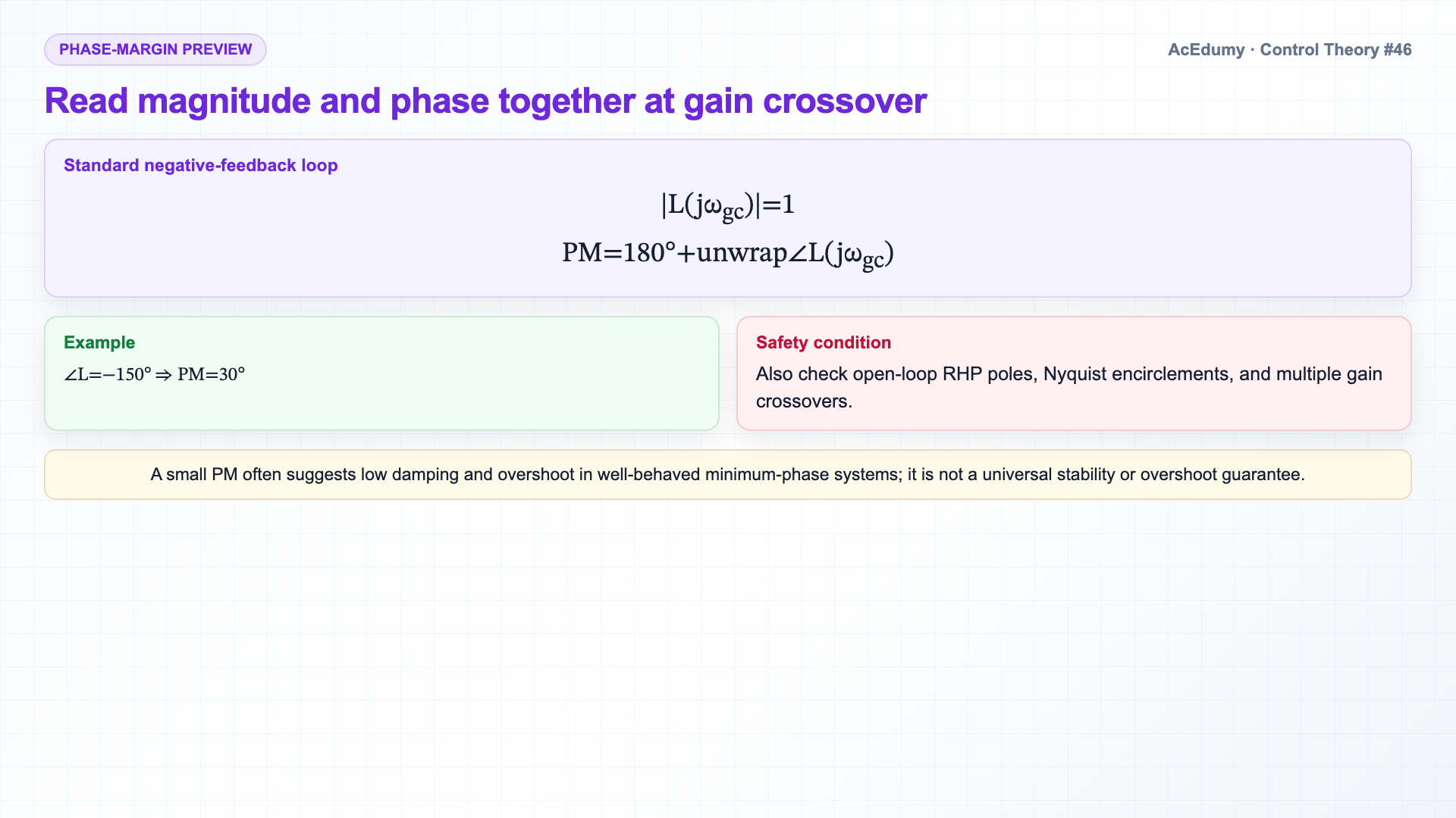
For G(s)=10/[s(s+1)(s+10)], exact phase is −90°−atan(ω)−atan(ω/10), while the asymptote moves from −90° to −270°.
One application worth previewing.
For a standard negative-feedback loop, gain crossover satisfies |L(jω_gc)|=1; phase margin uses the unwrapped loop phase there.
If unwrap∠L(jω_gc)=−150°, then PM=180°−150°=30°.
A small phase margin often suggests low damping and overshoot in well-behaved minimum-phase systems; it is not a universal guarantee.
Interpreting PM for stability also requires the open-loop RHP-pole count, Nyquist encirclements, and any multiple gain crossovers.
We will dig into gain and phase margins in two lectures.
For now, remember — a Bode phase plot is not just decorative.
Closed-loop robustness must be inferred from open-loop |L| and ∠L together with Nyquist conditions, not from phase alone.
Narration transcript
One application worth previewing. At the gain crossover frequency — where the magnitude curve crosses zero dB — the phase tells us how close to instability the closed loop is. If phase at gain crossover is, say, minus one hundred fifty degrees, the phase margin is one hundred eighty minus one hundred fifty equals thirty degrees. A small margin — the system is lightly damped, prone to overshoot. If phase at gain crossover is closer to minus one hundred eighty, the margin shrinks toward zero — and the closed loop teeters on instability. We will dig into gain and phase margins in two lectures. For now, remember — a Bode phase plot is not just decorative. It tells you, at every frequency, how stable a closed-loop system designed around that loop gain will be.
8. Summarize the Bode-phase results
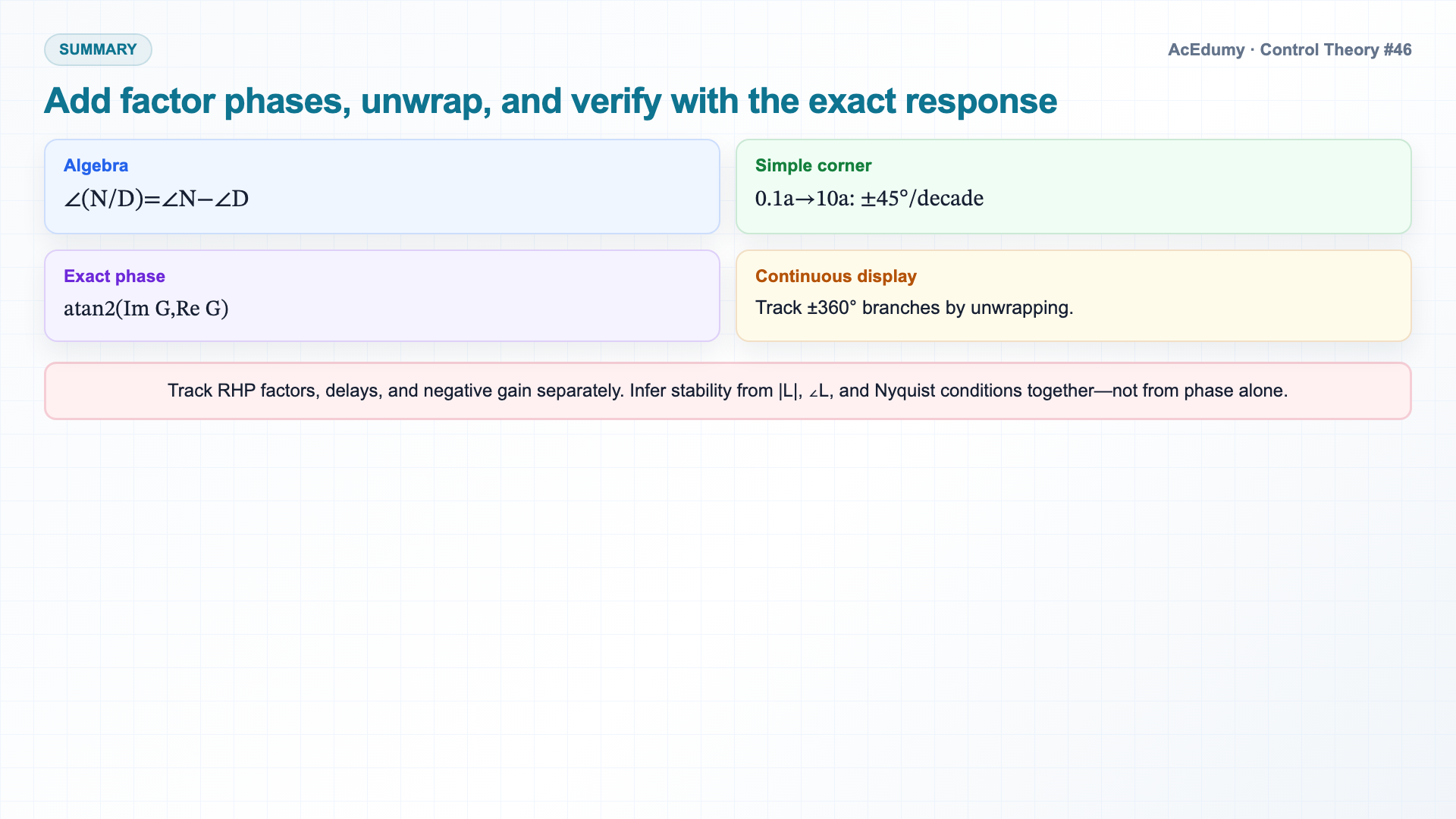
For G(s)=10/[s(s+1)(s+10)], exact phase is −90°−atan(ω)−atan(ω/10), while the asymptote moves from −90° to −270°.
Summary.
Bode phase plot — phase in degrees vs log frequency.
Total phase is the sum of factor phases.
Use the same atom decomposition as for magnitude.
Each atom has a known asymptotic phase: zero or one eighty for constants, plus or minus ninety for integrators and differentiators, smooth transition between zero and plus or minus ninety per simple pole or zero, double for complex pairs.
Decade rule — simple pole or zero ramps over two decades, with the corner at the midpoint.
Sum the contributions, draw the curve, read the system.
With magnitude and phase, the Bode plot is complete.
Next lecture we do a few full Bode examples — magnitude and phase together — and start to read what they tell us about stability and bandwidth.
Narration transcript
Summary. Bode phase plot — phase in degrees vs log frequency. Total phase is the sum of factor phases. Use the same atom decomposition as for magnitude. Each atom has a known asymptotic phase: zero or one eighty for constants, plus or minus ninety for integrators and differentiators, smooth transition between zero and plus or minus ninety per simple pole or zero, double for complex pairs. Decade rule — simple pole or zero ramps over two decades, with the corner at the midpoint. Sum the contributions, draw the curve, read the system. With magnitude and phase, the Bode plot is complete. Next lecture we do a few full Bode examples — magnitude and phase together — and start to read what they tell us about stability and bandwidth.