#09 Line, surface, and volume charge densities; fields of an infinite line, infinite sheet, and charged ring

Below are all the lines written in the notebook together with the full narration transcript.

1. 1. Move from point charges to continuous charge

   

   In our last lesson, we learned Coulomb's law and the electric field due to point charges.

   We used the superposition principle to add up contributions from multiple charges.

   But real-world charges are rarely isolated points.

   A charged wire, a metal plate, a cloud of electrons — these are all continuous distributions of charge.

   Today, we'll learn how to find the electric field when charge is spread along a line, across a surface, or throughout a volume.

   Narration transcript

   In our last lesson, we learned Coulomb's law and the electric field due to point charges. We used the superposition principle to add up contributions from multiple charges. But real-world charges are rarely isolated points. A charged wire, a metal plate, a cloud of electrons — these are all continuous distributions of charge. Today, we'll learn how to find the electric field when charge is spread along a line, across a surface, or throughout a volume.

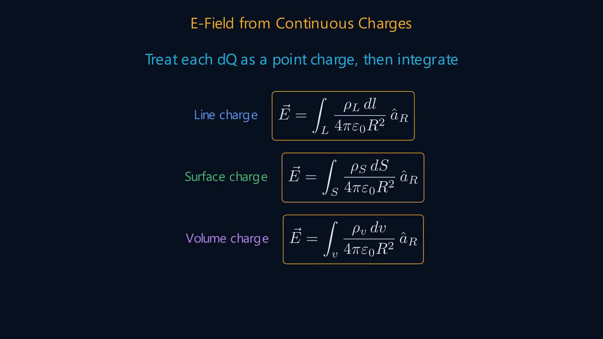
2. 2. Define three charge densities and integrals

   

   There are three types of continuous charge distributions, and each one has its own charge density.

   First, line charge density, ρ_L.

   This describes charge spread along a thin wire or line.

   It's measured in coulombs per meter.

   Total line charge: Q = ∫ₗ ρ_L dl.

   Second, surface charge density, ρ_S.

   This describes charge spread across a flat or curved surface.

   It's measured in coulombs per square meter.

   Total surface charge: Q = ∫ₛ ρ_S dS.

   Third, volume charge density, ρ_v.

   This describes charge filling a three-dimensional region.

   It's measured in coulombs per cubic meter.

   Total volume charge: Q = ∫ᵥ ρ_v dv.

   Now, to find the electric field from any of these distributions, we use a powerful idea: treat each tiny piece of charge dQ as a point charge.

   Write its contribution to the field using Coulomb's law, then integrate over the entire distribution.

   This gives us three integral formulas.

   For a line charge, E = ∫[ρ_L dl/(4πε₀R²)]e_R.

   For a surface charge: replace ρ_L dl with ρ_S dS.

   And for a volume charge: replace it with ρ_v dv.

   These three formulas are the foundation for everything in this lesson.

   Narration transcript

   There are three types of continuous charge distributions, and each one has its own charge density. First, line charge density, rho-L. This describes charge spread along a thin wire or line. It's measured in coulombs per meter. The total charge on the line is the integral of rho-L d-l over the length of the line. Second, surface charge density, rho-S. This describes charge spread across a flat or curved surface. It's measured in coulombs per square meter. The total charge is the integral of rho-S d-S over the surface. Third, volume charge density, rho-v. This describes charge filling a three-dimensional region. It's measured in coulombs per cubic meter. The total charge is the integral of rho-v d-v over the volume. Now, to find the electric field from any of these distributions, we use a powerful idea: treat each tiny piece of charge d-Q as a point charge. Write its contribution to the field using Coulomb's law, then integrate over the entire distribution. This gives us three integral formulas. For a line charge: E equals the integral of rho-L d-l over four pi epsilon-zero R-squared, in the direction of a-R. For a surface charge: replace rho-L d-l with rho-S d-S. And for a volume charge: replace it with rho-v d-v. These three formulas are the foundation for everything in this lesson.

3. 3. Derive the infinite-line field

   

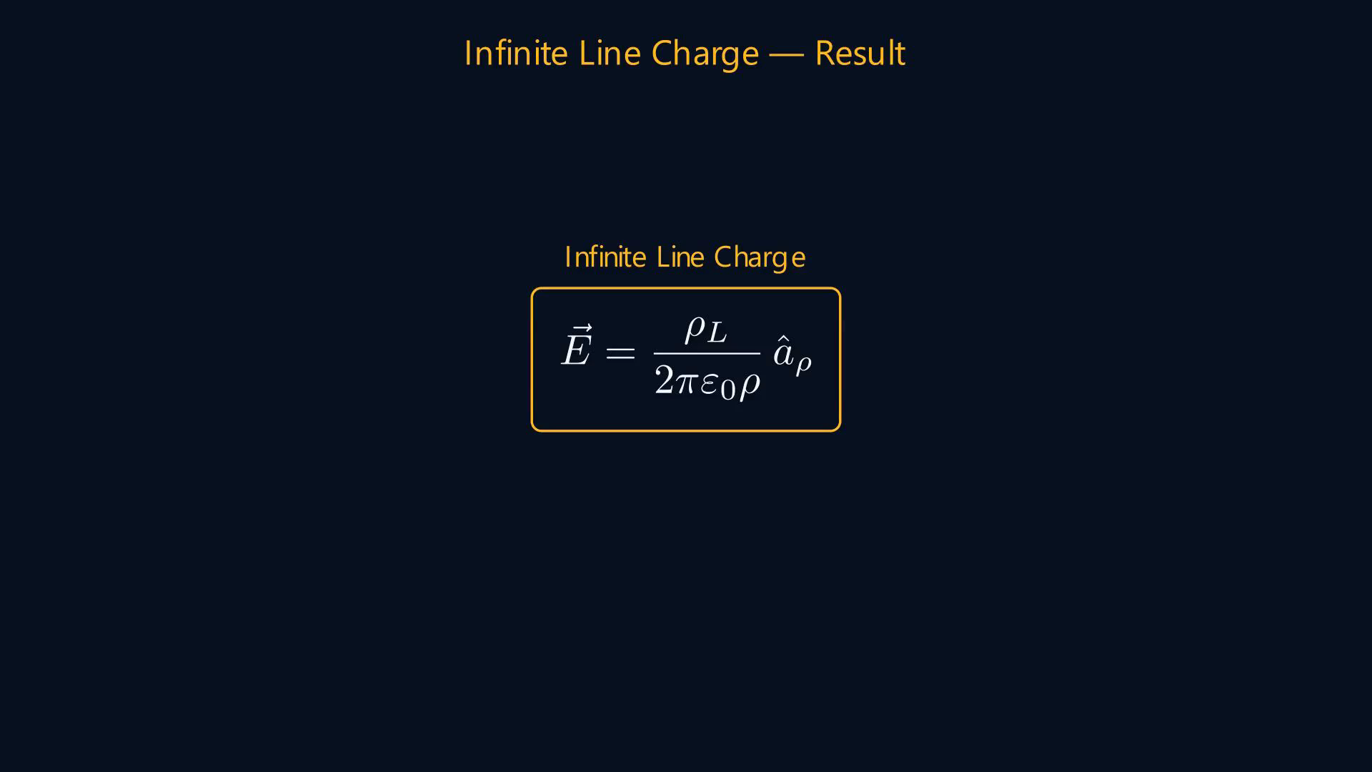
   Let's apply the line charge formula to an important case: an infinite line of charge along the z-axis, with uniform charge density ρ_L.

   We want the electric field at a point P located at perpendicular distance ρ from the z-axis.

   Consider a small element dl at position z′ on the line.

   The element carries dQ = ρ_L dz′.

   The vector R from this element to point P has two components: ρ in the radial direction, and z minus z′ in the z-direction.

   The distance relation is R² = ρ² + (z − z′)².

   Now here's a key insight from symmetry.

   For every element at plus z′, there's a matching element at minus z′.

   Their radial components add up, but their z-components cancel.

   So the total field has only a ρ-component.

   To evaluate the integral, we use a trigonometric substitution.

   Use the substitution z′ = −ρ tan α.

   After working through the calculus — substituting, simplifying, and integrating from minus infinity to plus infinity — we arrive at a beautifully simple result:

   Infinite line charge:

   $\displaystyle E = \left[\frac{\rho _{L}}{2\pi \varepsilon ₀\rho }\right]e_{\rho }.$

   This is worth memorizing.

   The electric field of an infinite line charge drops off as one over ρ — not one over ρ² like a point charge.

   And the field points radially outward, perpendicular to the wire.

   Narration transcript

   Let's apply the line charge formula to an important case: an infinite line of charge along the z-axis, with uniform charge density rho-L. We want the electric field at a point P located at perpendicular distance rho from the z-axis. Consider a small element d-l at position z-prime on the line. This element carries charge d-Q equals rho-L d-z-prime. The vector R from this element to point P has two components: rho in the radial direction, and z minus z-prime in the z-direction. So R-squared equals rho-squared plus z minus z-prime, squared. Now here's a key insight from symmetry. For every element at plus z-prime, there's a matching element at minus z-prime. Their radial components add up, but their z-components cancel. So the total field has only a rho-component. To evaluate the integral, we use a trigonometric substitution. Let z-prime equal minus rho times tangent alpha. After working through the calculus — substituting, simplifying, and integrating from minus infinity to plus infinity — we arrive at a beautifully simple result: E equals rho-L over two pi epsilon-zero rho, in the a-rho direction. This is worth memorizing. The electric field of an infinite line charge drops off as one over rho — not one over rho-squared like a point charge. And the field points radially outward, perpendicular to the wire.

4. 4. Calculate the infinite-sheet field

   

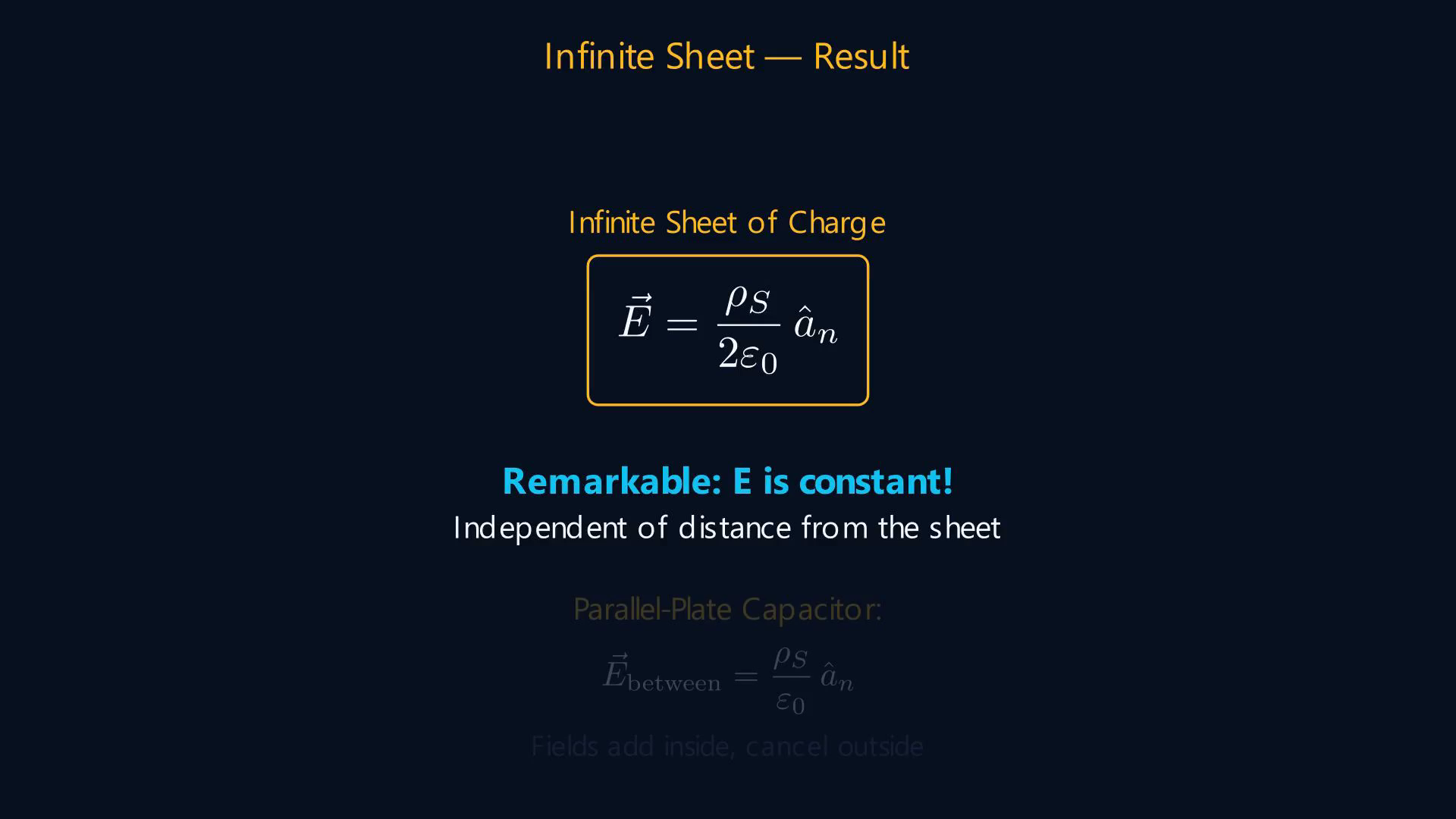
   Now let's find the field due to an infinite sheet of charge in the x-y plane, with uniform surface charge density ρ_S.

   We want the field at point P, located at height h above the sheet.

   Consider a small element dS at position ρ, φ on the sheet.

   The differential charge is dQ = ρ_S ρ dρ dφ.

   The vector R from dS to point P has a radial component minus e_ρ and a vertical component h times e_z.

   Again, symmetry saves us.

   For every element at angle φ, there's one at φ plus π.

   Their horizontal components cancel.

   Only the z-component survives.

   So we integrate only E-z.

   Setting up the integral in cylindrical coordinates and integrating ρ from zero to infinity and φ from zero to two-π, we get:

   Infinite sheet:

   $\displaystyle E = \left[\frac{\rho _{S}}{2\varepsilon ₀}\right]e_{z}.$

   This result is remarkable.

   The electric field of an infinite sheet is constant — it doesn't depend on the distance from the sheet at all!

   Whether you're one centimeter or one kilometer away, the field strength is the same.

   Between parallel plates E = ρ_S/ε₀; the fields cancel outside.

   Narration transcript

   Now let's find the field due to an infinite sheet of charge in the x-y plane, with uniform surface charge density rho-S. We want the field at point P, located at height h above the sheet. Consider a small element d-S at position rho, phi on the sheet. It carries charge d-Q equals rho-S times rho d-rho d-phi. The vector R from d-S to point P has a radial component minus a-rho and a vertical component h times a-z. Again, symmetry saves us. For every element at angle phi, there's one at phi plus pi. Their horizontal components cancel. Only the z-component survives. So we integrate only E-z. Setting up the integral in cylindrical coordinates and integrating rho from zero to infinity and phi from zero to two-pi, we get: E equals rho-S over two epsilon-zero, in the a-z direction. This result is remarkable. The electric field of an infinite sheet is constant — it doesn't depend on the distance from the sheet at all! Whether you're one centimeter or one kilometer away, the field strength is the same. For a parallel-plate capacitor with equal and opposite charges, the fields add between the plates, giving E equals rho-S over epsilon-zero, and cancel outside.

5. 5. Find the axial field of a charged ring

   

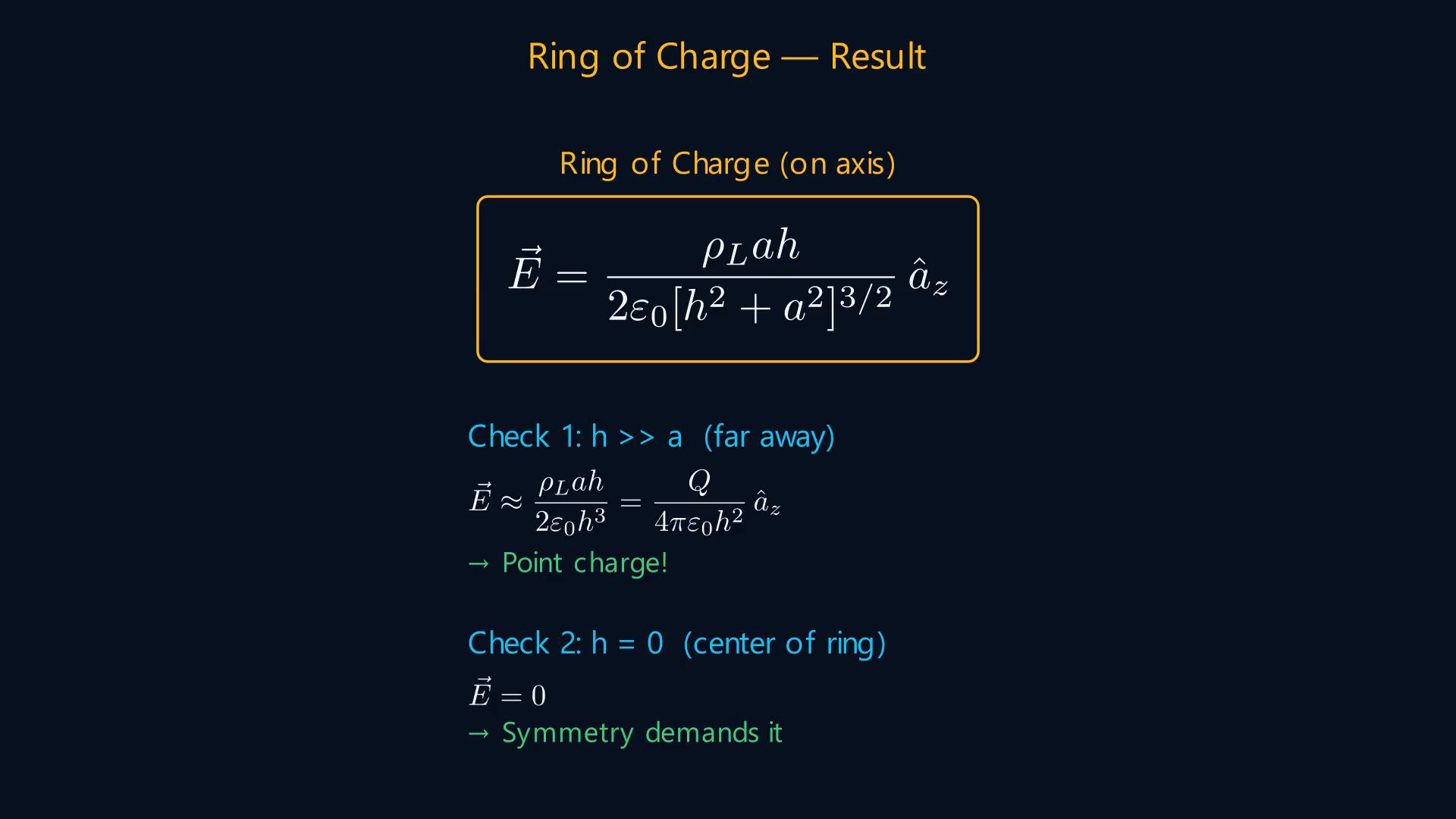
   Let's work through an important example.

   A circular ring of radius a carries a uniform line charge ρ_L.

   The ring lies in the x-y plane, centered at the origin.

   We want the field at point P on the z-axis, at height h.

   For a ring element, dl = a dφ and dQ = ρ_L a dφ.

   For every element, R = √(a² + h²).

   This is the same for every element on the ring, which makes the integration simpler.

   The vector R from an element to P has components minus a in the e_ρ direction, and h in the e_z direction.

   By symmetry, the horizontal components cancel — for every element, there's one on the opposite side of the ring that cancels its radial contribution.

   Only the z-component survives.

   Integrating around the ring from zero to two-π, we get:

   On the ring axis, E = [ρ_L a h/(2ε₀(h² + a²)⁽3/2))]e_z.

   For h ≫ a, the ring behaves like a point charge: E → Q/(4πε₀h²).

   At the ring center, h = 0 and E = 0.

   Narration transcript

   Let's work through an important example. A circular ring of radius a carries a uniform line charge rho-L. The ring lies in the x-y plane, centered at the origin. We want the field at point P on the z-axis, at height h. Each small element d-l equals a d-phi carries charge d-Q equals rho-L times a d-phi. The distance from any element to P is R equals the square root of a-squared plus h-squared. This is the same for every element on the ring, which makes the integration simpler. The vector R from an element to P has components minus a in the a-rho direction, and h in the a-z direction. By symmetry, the horizontal components cancel — for every element, there's one on the opposite side of the ring that cancels its radial contribution. Only the z-component survives. Integrating around the ring from zero to two-pi, we get: E equals rho-L times a times h, divided by two epsilon-zero times the quantity h-squared plus a-squared, to the three-halves power, all in the a-z direction. Two important checks: when h is much larger than a, the ring looks like a point charge, and indeed the formula reduces to Q over four pi epsilon-zero h-squared. And when h equals zero — at the center of the ring — the field is zero, as symmetry demands.

6. 6. Review symmetry results and limits

   

   Let's recap the three key results from today.

   Infinite line: E = ρ_L/(2πε₀ρ), decreasing as 1/ρ.

   Infinite sheet: E = ρ_S/(2ε₀), a constant.

   Charged ring axis:

   $\displaystyle E = \rho _{L} a h/\left[2\varepsilon ₀\left(h² + a²\right)^{(}3/2)\right].$

   The common technique in all three: exploit symmetry to identify which components cancel, then integrate what remains.

   Next time, we'll introduce the electric flux density vector D, which simplifies how we handle materials and leads directly to Gauss's law.

   Narration transcript

   Let's recap the three key results from today. An infinite line charge produces a field that drops off as one over rho: E equals rho-L over two pi epsilon-zero rho. An infinite sheet of charge produces a constant field: E equals rho-S over two epsilon-zero. And a charged ring produces a field along its axis: E equals rho-L a h over two epsilon-zero times h-squared plus a-squared to the three-halves. The common technique in all three: exploit symmetry to identify which components cancel, then integrate what remains. Next time, we'll introduce the electric flux density vector D, which simplifies how we handle materials and leads directly to Gauss's law.

Source video: Electromagnetic Theory (v2) #09 Continuous Charge Distributions & E Field (8:10)