Control Theory · Active Suspension Modeling

#24 Model the signed control and road forces and build the two-integrator suspension plant

Derive an ideal suspension plant from its force balance and keep both inputs, the restoring sign and the initial states explicit.

Question

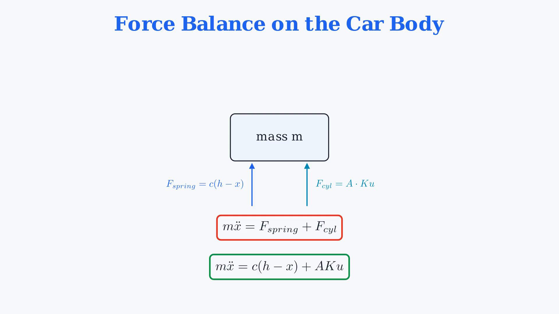
Existing final-video frame showing suspension signals, incremental forces, the motion equation, integrators or the signed plant block diagram. — Read all displacements and forces as increments about loaded static equilibrium. The opening section uses the existing force card, and the summary uses the existing equation card. The spring return branch represents the restoring force; a controller has not yet been designed.

Model an ideal single-degree-of-freedom sprung car-body mass m, supported by a linear spring of stiffness c and an ideal hydraulic actuator of effective piston area A. Take m, c and A positive. Here c is spring stiffness, not a viscous damping coefficient. The wheel or base is assumed to follow the prescribed road height h; wheel mass, tire compliance, damping, friction, actuator dynamics, delays and saturation are omitted. This is a defined plant idealization for later controller design, not a full physical car model. Choose upward displacement and force as positive. Measure body displacement x and road displacement h from the loaded static equilibrium. The narration's spring rest position means this loaded equilibrium, not the spring's unloaded natural length. If the static spring compression is d0 and the static actuator voltage is u0, the equilibrium balance is c d0 + A K u0 = m g. The physical spring compression after a perturbation is d0+h-x. With zero actuator bias, d0=m g/c. Define u as the voltage increment about u0. For the ideal converter, the incremental pressure difference is delta p=K u; the actuator orientation and signed gain K are chosen so that positive K u produces positive upward force. Pressure difference, voltage and actuator force can therefore be signed increments. The total physical force equation contains the spring preload and weight. Subtract the static equilibrium balance to obtain m x''=c(h-x)+A K u. Thus gravity remains a real force; it disappears only from the incremental equation because its equilibrium contribution has already been balanced. The incremental spring force is c(h-x), not c h-x: stiffness multiplies the entire relative displacement. This grouping is explicit in the source's expanded equation. The summary's abbreviated spoken expression must be read with those same parentheses. Positive h increases the upward spring force; positive x decreases it. The force-card arrows mark reference directions and do not assert that both forces are positive at every instant. Expand and rearrange as m x''=c h-c x+A K u and m x''+c x=c h+A K u. There are two independent excitation signals, control voltage u and prescribed road disturbance h, and one measured output x. Body mass is in kilograms, displacement in meters, c in newtons per meter, A in square meters, K in pascals per volt, and delta p in pascals. Both c(h-x) and A K u have units of newtons. The source supplies no numerical parameter values. Build the forward force path from voltage through K, then A, into the positive summing input. Road height passes through c into a separate positive input. Body displacement is taken after the second integrator and returned through c into the negative input. The force sum F_sum equals c h-c x+A K u. Divide the complete sum by m to obtain acceleration a, then integrate once to velocity v and once more to displacement x. Do not put only one force term under the mass factor. The integrators must retain their initial states: v(t)=v0+the integral of a from zero to t, and x(t)=x0+the integral of v from zero to t. Equivalently x'=v and v'=-(c/m)x+(c/m)h+(A K/m)u. Two integrators require two specified initial conditions. A bare 1/s block denotes zero initial state unless its stored initial value is separately supplied. For zero initial conditions only, the Laplace relation is (m s squared+c)X=c H+A K U. The control-to-displacement transfer is A K/(m s squared+c) with the road input set to zero; the road-to-displacement transfer is c/(m s squared+c) with the voltage input set to zero. Superposition adds their responses and the initial-state response when applicable. A one-input transfer alone does not describe the whole two-input plant. The negative spring return path models the mechanical restoring relation; it is not a designed feedback controller. Keeping x close to zero despite h is the control objective, not an achieved property of the diagram. Since no damping is present, the poles lie at plus and minus j times square root of c/m. Free oscillations persist. The unforced ideal plant is not asymptotically stable, and it is not BIBO stable: bounded sinusoidal forcing at its natural frequency produces a growing resonant response. With constant inputs, a possible equilibrium satisfies c x=c h+A K u, but an arbitrary trajectory does not necessarily settle there. Do not use the final-value theorem to claim settling for this undamped plant. A controller and a more detailed physical model can be considered in subsequent design work.

Written solution and narration transcript(shows the full solution)

Below are all the lines written in the notebook together with the full narration transcript.

1. Define the ideal suspension plant
Read all displacements and forces as increments about loaded static equilibrium. The opening section uses the existing force card, and the summary uses the existing equation card. The spring return branch represents the restoring force; a controller has not yet been designed.
Define the ideal suspension plant.
Treat road height as a prescribed base displacement.
Use body mass m and positive spring stiffness c; damping is omitted.
The ideal hydraulic actuator has effective piston area A.
Incremental converter relation:
$\displaystyle \Delta p = K\cdot u$
The later control objective is to keep body displacement near zero despite road changes.
Identify the signals, derive the incremental equation and build the plant diagram.
Narration transcript
Here is the problem. We have a car driving on a bumpy road. The car body has mass m and sits on a spring with spring constant c. There is also a hydraulic cylinder with surface area A that can push the body up or down. An electro hydraulic converter takes an input voltage u and creates a pressure difference delta p equals K times u. The goal of the system is to keep the car body steady, meaning displacement x should stay close to zero, even when the road surface height h changes. We need to do three things: identify the input, output, and disturbance signals; write the differential equation; and draw the block diagram.
2. Identify control and disturbance signals
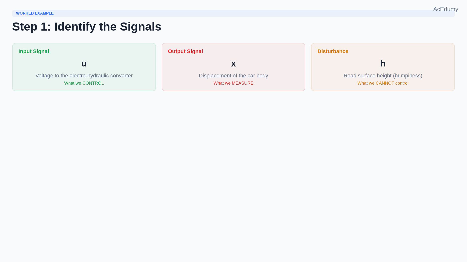
Read all displacements and forces as increments about loaded static equilibrium. The opening section uses the existing force card, and the summary uses the existing equation card. The spring return branch represents the restoring force; a controller has not yet been designed.
Classify the signals before deriving the model.
Choose the manipulated variable.
The voltage increment u drives the ideal converter.
Treat u as the control input.
Choose the quantity to be regulated.
Use body displacement x measured from loaded equilibrium.
Treat x as the output.
Identify the externally imposed excitation.
Use prescribed road-height displacement h.
Treat h as a disturbance input.
Retain both inputs u and h and the output x.
Narration transcript
Let us start with part a: identifying the signals. What can we control? The voltage u going into the electro hydraulic converter. That is our input signal. What do we want to measure or regulate? The displacement x of the car body. That is our output signal. What is the external disturbance we cannot control? The bumpiness of the road, which is the height h. That is our disturbance signal. So to summarize: input is u, output is x, disturbance is h.
3. Balance incremental forces
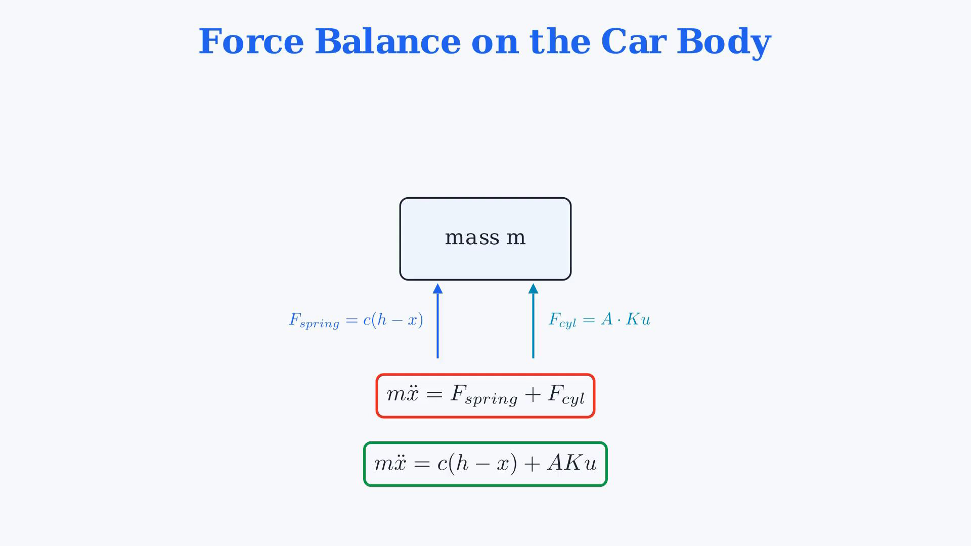
Read all displacements and forces as increments about loaded static equilibrium. The opening section uses the existing force card, and the summary uses the existing equation card. The spring return branch represents the restoring force; a controller has not yet been designed.
Derive the force balance with an upward-positive convention.
Apply Newton's second law to the body mass.
Net force equals mass times acceleration.
Newton equation:
$\displaystyle m\cdot x''\left(t\right) = F_{\mathrm{sum}}\left(t\right)$
List the physical forces before subtracting equilibrium.
Include the spring, actuator and weight.
Start with the incremental spring force.
The ideal wheel or base follows h.
Incremental compression:
$\displaystyle \Delta d = h-x$
Incremental spring force:
$\displaystyle F_{\mathrm{spring}} = c\cdot \left(h-x\right)$
Next include the signed actuator force.
Pressure-to-force relation:
$\displaystyle F_{\mathrm{cyl}} = A\cdot \Delta p$
Incremental converter relation:
$\displaystyle \Delta p = K\cdot u$
Actuator force:
$\displaystyle F_{\mathrm{cyl}} = A\cdot K\cdot u$
The loaded static spring and any actuator bias balance weight; an unloaded spring reference would not remove gravity.
Subtract the loaded equilibrium balance; weight then cancels from the incremental equation.
Narration transcript
Now part b: the differential equation. We use Newton's second law. The sum of all forces on the car body equals mass times acceleration. Let us write m times x double dot equals the sum of forces, F sigma. What forces act on the car body? Three forces. First, the spring force. The spring connects the car body to the wheel. When the road goes up by h and the body moves up by x, the spring compression is h minus x. So the spring force is c times h minus x. Second, the hydraulic cylinder force. The cylinder pushes with a force equal to the pressure difference times the surface area: A times delta p. And we know delta p equals K times u. So the cylinder force is A times K times u. Third, gravity pulls down with force m times g, and the spring rest position already accounts for gravity. So when we write the spring force as c times h minus x, gravity cancels out.
4. Rearrange the equation of motion
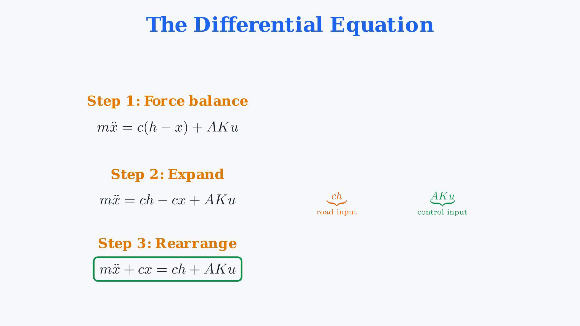
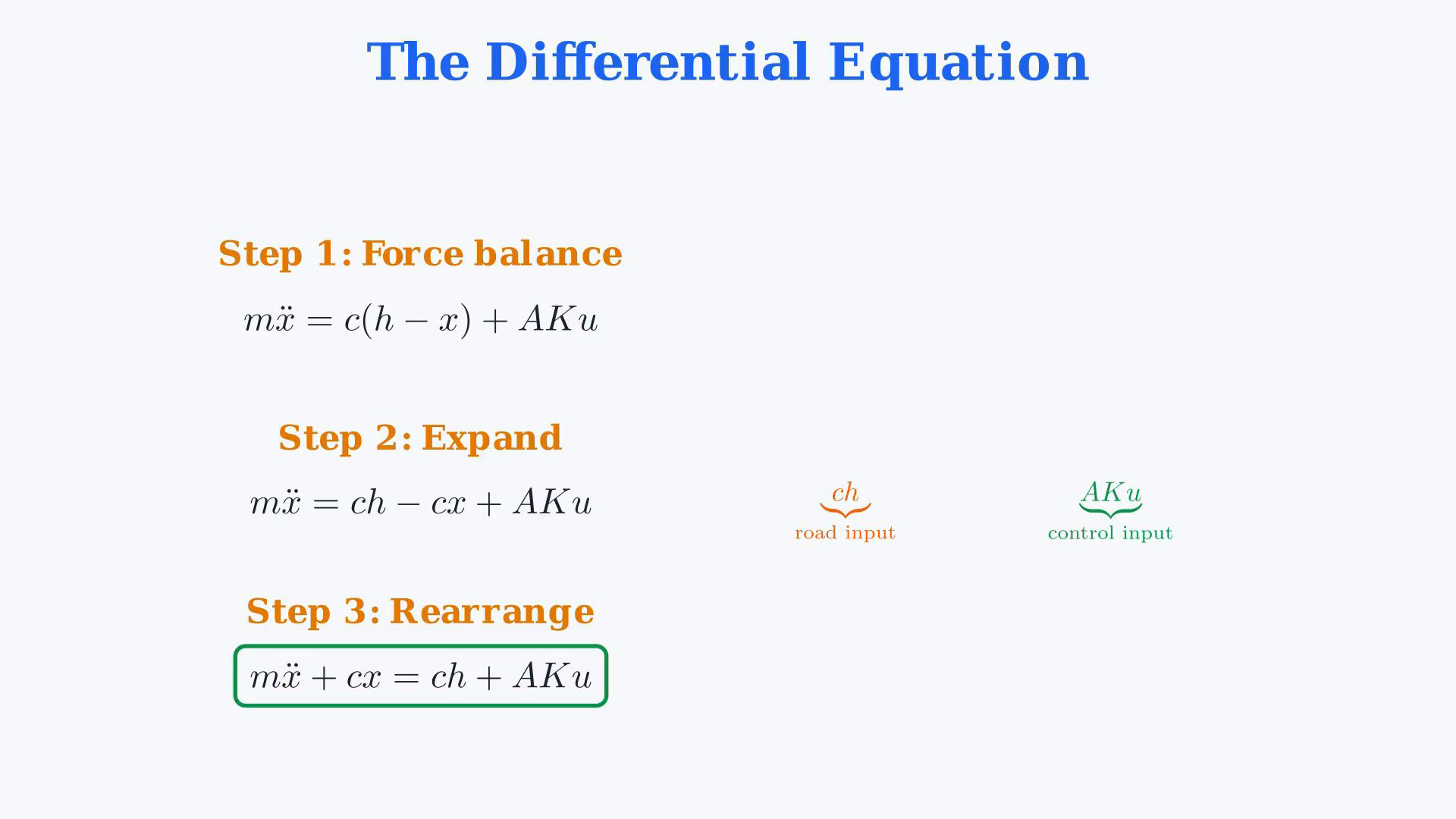
Read all displacements and forces as increments about loaded static equilibrium. The opening section uses the existing force card, and the summary uses the existing equation card. The spring return branch represents the restoring force; a controller has not yet been designed.
Combine the two incremental forces.
Grouped force balance:
$\displaystyle m\cdot x''\left(t\right) = c\cdot \left(h\left(t\right)-x\left(t\right)\right)+A\cdot K\cdot u\left(t\right)$
Expanded force balance:
$\displaystyle m\cdot x''\left(t\right) = c\cdot h\left(t\right)-c\cdot x\left(t\right)+A\cdot K\cdot u\left(t\right)$
This is the equation for the stated undamped idealization.
Keep road displacement h and voltage u as independent inputs.
The body displacement x is the output.
Rearranged plant equation:
$\displaystyle m\cdot x''\left(t\right)+c\cdot x\left(t\right) = c\cdot h\left(t\right)+A\cdot K\cdot u\left(t\right)$
Narration transcript
Putting it all together. m times x double dot equals c times the quantity h minus x, plus A times K times u. Let us expand: m times x double dot equals c times h minus c times x plus A times K times u. This is our differential equation. Notice it has two inputs: the disturbance h from the road, and the control input u from the voltage. The output is x, the displacement. Let us rearrange: m times x double dot plus c times x equals c times h plus A times K times u.
5. Include the two state integrators
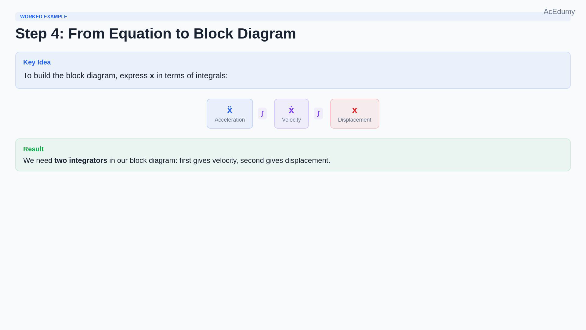
Read all displacements and forces as increments about loaded static equilibrium. The opening section uses the existing force card, and the summary uses the existing equation card. The spring return branch represents the restoring force; a controller has not yet been designed.
Construct the two integrators with their initial states.
Acceleration:
$\displaystyle a\left(t\right) =\frac{c\cdot h\left(t\right)-c\cdot x\left(t\right)+A\cdot K\cdot u\left(t\right)}{m}$
Velocity with initial value:
$\displaystyle v\left(t\right) = v_{0}+\int _{0}^{t} a\left(\tau \right) \mathrm{d}\tau$
Displacement with initial value:
$\displaystyle x\left(t\right) = x_{0}+\int _{0}^{t} v\left(\tau \right) \mathrm{d}\tau$
The two states are velocity and displacement.
The first integrator accumulates acceleration and starts at the specified initial velocity.
The second accumulates velocity and starts at the specified initial displacement.
Narration transcript
To build the block diagram, we need to express x in terms of integrals. From the equation, x double dot equals one over m times the quantity c times h minus c times x plus A times K times u. If we integrate x double dot once, we get x dot, the velocity. If we integrate again, we get x, the displacement. So we need two integrators in our block diagram. The first integrator takes the acceleration and gives velocity. The second takes velocity and gives displacement.
6. Preserve the signed force summation
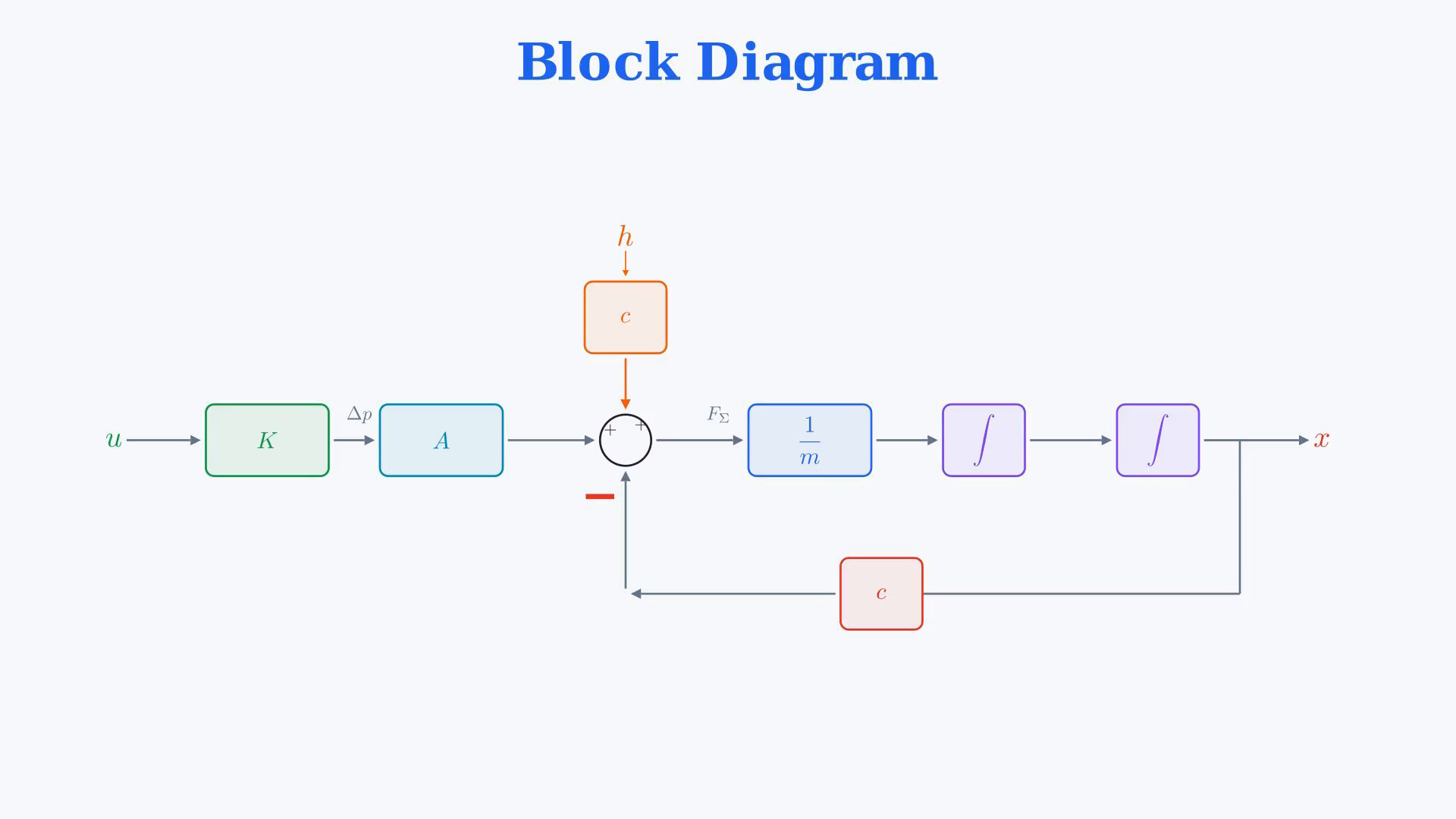
Read all displacements and forces as increments about loaded static equilibrium. The opening section uses the existing force card, and the summary uses the existing equation card. The spring return branch represents the restoring force; a controller has not yet been designed.
Build the signed plant interconnection.
Follow the voltage branch from left to right.
Incremental converter relation:
$\displaystyle \Delta p = K\cdot u$
Pressure-to-force relation:
$\displaystyle F_{\mathrm{cyl}} = A\cdot \Delta p$
Enter the actuator force at a positive summing input.
Road contribution:
$\displaystyle F_{\mathrm{road}} = c\cdot h$
Enter the road contribution at its own positive summing input.
The body-displacement branch has magnitude c times x and must be subtracted.
Restoring contribution:
$\displaystyle F_{\mathrm{return}} = -c\cdot x$
Force sum:
$\displaystyle F_{\mathrm{sum}} = c\cdot h-c\cdot x+A\cdot K\cdot u$
Acceleration:
$\displaystyle a =\frac{ F_{\mathrm{sum}}}{m}$
Integrate acceleration to velocity, retaining its initial value.
Integrate velocity to displacement, retaining its initial value.
Take x after the second integrator and return it through c to the negative summing input.
Narration transcript
Now let us draw the block diagram step by step. Start from the left. The input voltage u goes through a block K, giving delta p. Then through a block A, giving the cylinder force A times delta p. This force enters a summing junction. The road disturbance h goes through a block c, giving the spring force from the road: c times h. This also enters the summing junction as a positive input. The spring force from the body displacement is c times x. This enters as a negative feedback: minus c times x. The sum of these forces is F sigma. F sigma goes through a block one over m, giving the acceleration. Then through the first integrator, giving velocity. Then through the second integrator, giving the output x. Finally, x feeds back through a block c to create the negative spring force feedback.
7. Review the plant model
Read all displacements and forces as increments about loaded static equilibrium. The opening section uses the existing force card, and the summary uses the existing equation card. The spring return branch represents the restoring force; a controller has not yet been designed.
Review the scope and signs of the model.
Use the ideal body mass, spring and hydraulic actuator about loaded equilibrium.
Control voltage u and road height h drive the displacement output x.
Incremental plant equation:
$\displaystyle m\cdot x''\left(t\right) = c\cdot \left(h\left(t\right)-x\left(t\right)\right)+A\cdot K\cdot u\left(t\right)$
The two input paths, signed spring return and two initial-state integrators reproduce the force balance.
The plant is ready for later controller design; this undamped model does not yet achieve the regulation objective.
Narration transcript
Let us review what we did. We started with a physical system: a car on a bumpy road with a spring and hydraulic actuator. We identified three signals: input voltage u, output displacement x, and disturbance road height h. We applied Newton's second law to write the differential equation: m x double dot equals c times h minus x plus A K u. And we translated this equation into a block diagram with two integrators, a feedback loop for the spring, and two input paths for the control voltage and the road disturbance. This is a complete plant model ready for controller design.