Control Theory · Block Diagram Simplification

#14 Preserve signed input-output relations when reducing series, parallel and feedback connections

Reduce signed connections and separate the motor voltage-to-speed and load-to-speed transfer functions.

Question

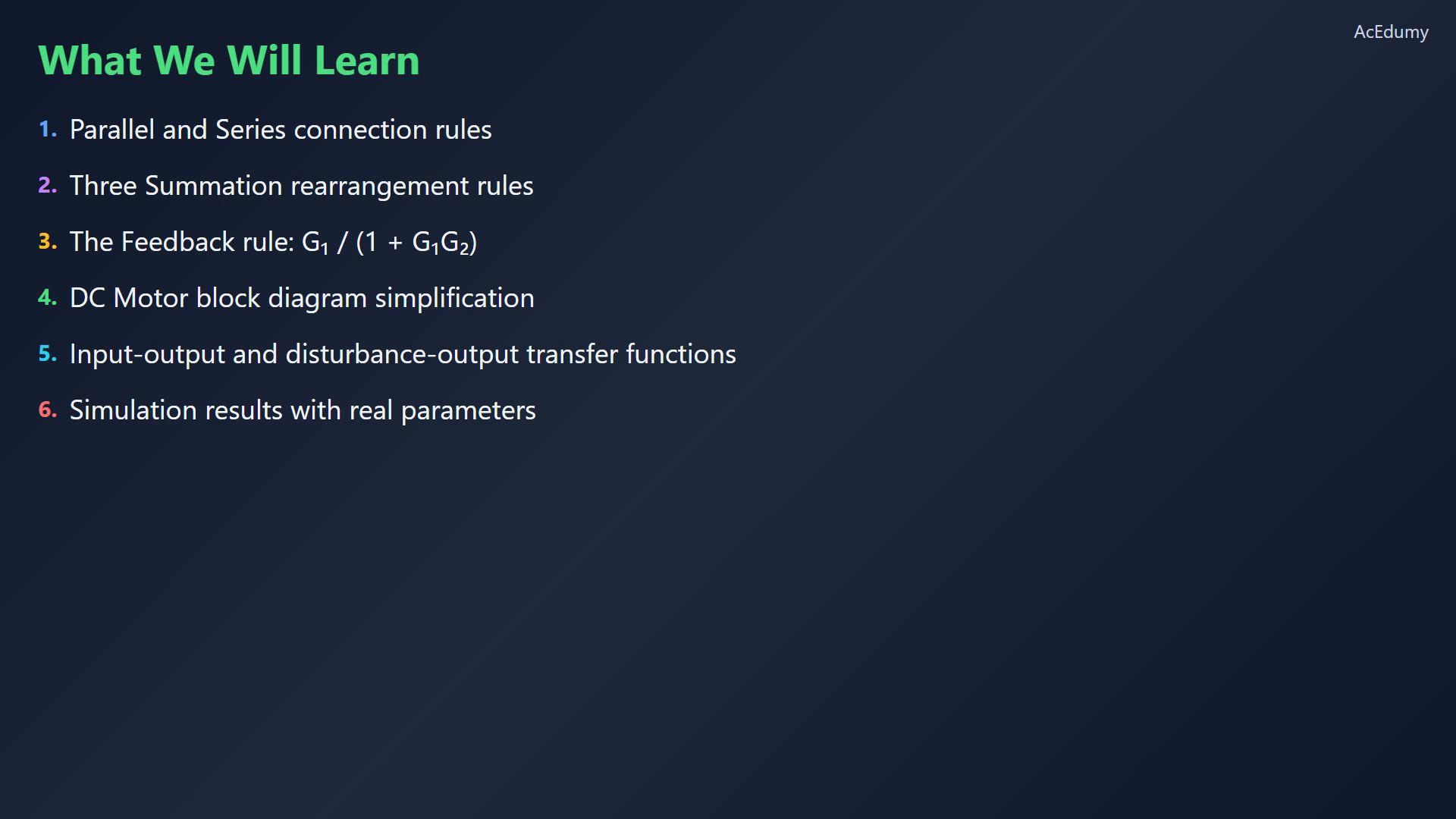
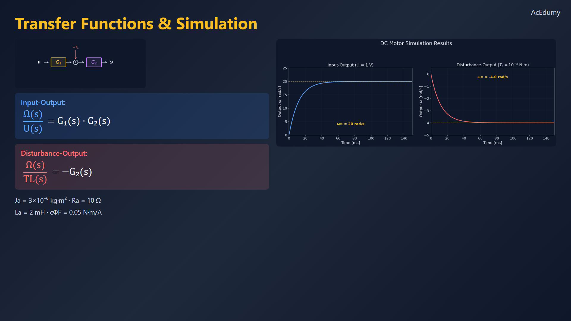
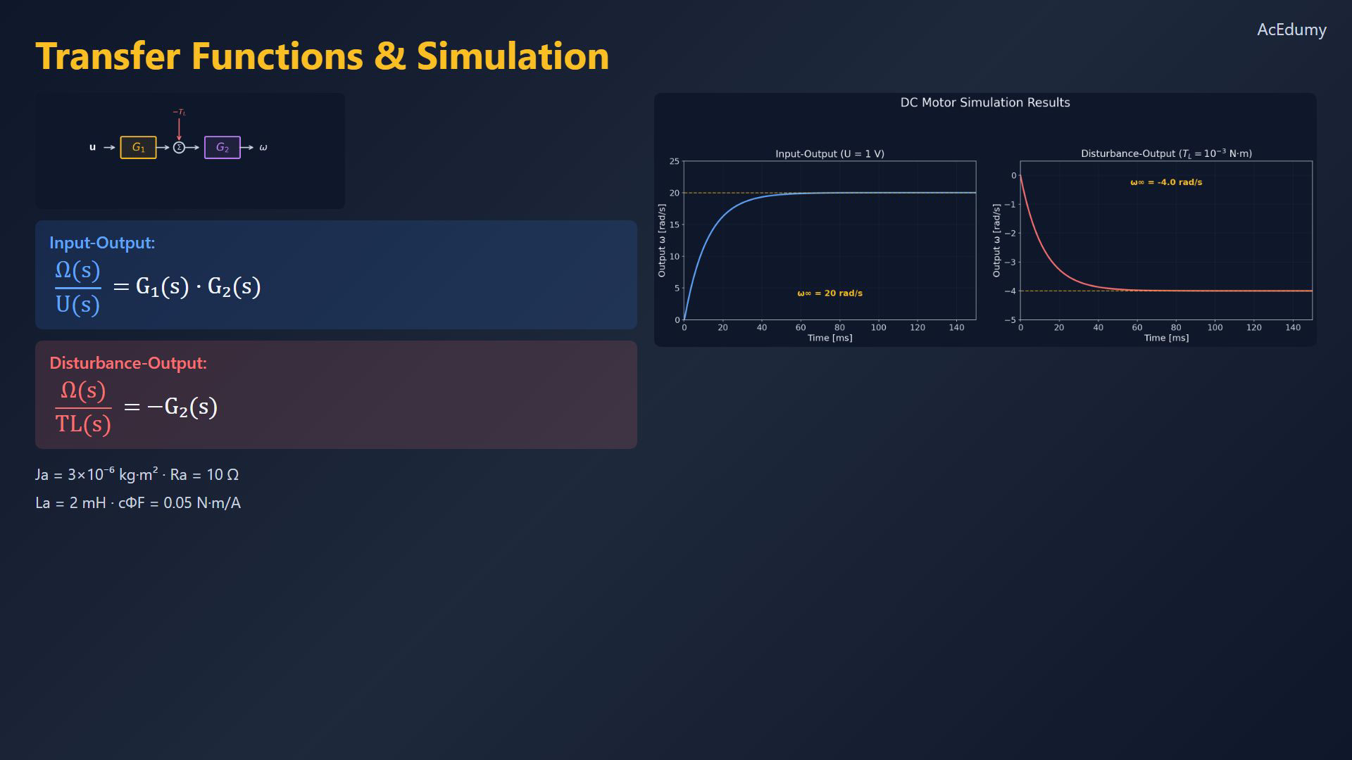
Existing lesson frame with a summation identity, feedback reduction or the motor voltage and load channels. — Use scalar zero-state LTI transfer relations. Parallel connections use the summation identity card; the full motor and outer-loop drawing use the final two-input result as an algebraic reference. The motor plots show separate 1 V voltage and 0.001 N m load steps with the other input zero. Define K as the whole fixed motor coupling c phi F.

Work with continuous-time scalar SISO LTI blocks in the zero state. Signals in transfer equations are Laplace transforms; nonzero initial conditions require separate initial-state terms. Parallel paths receive the same input and their distinct outputs enter an explicit signed summation. Two positive branches give G1+G2. In a cascade with G1 first and G2 second the ordered product is G2 G1; scalar transfer functions commute, so it is also G1 G2 here. Matrix-valued systems generally do not commute and require compatible dimensions. For linear G, distributing a sum gives G(u1+u2)=Gu1+Gu2. Moving an added u2 from after G to before it requires its factor 1/G. This is a formal identity only where the inverse exists: G must be nonzero, and a physical inverse need not be causal, proper or stable. An integrator inverse is a differentiator; a nonminimum-phase zero becomes an unstable inverse pole. Do not assume this rearrangement always provides a realizable block. Associativity permits regrouping the same signed additions. It does not permit moving junctions across intervening gains, delays or dynamics without the corresponding transformation. Preserve every branch and its sign. With negative feedback the error is u-G2 y and y=G1(u-G2 y), giving y(1+G1 G2)=G1 u and closed-loop gain G1/(1+G1 G2). Positive feedback instead gives G1/(1-G1 G2). These identities require a well-posed interconnection and an invertible denominator; a zero denominator cannot be divided away. For example static G1=G2=1 with positive feedback does not determine a unique output. Negative feedback alone does not guarantee stability. Check poles and internal modes; cancellations in one external transfer can hide internal instability. For the separately excited ideal DC motor use the same fixed coupling coefficient in the torque and back-EMF equations in consistent SI units. Define K as the whole source quantity c phi F, with fixed field flux; F is not an additional time-varying input. K squared means the square of that entire coefficient, not c times only flux squared or a separate F squared. The source uses compact cPhiF typography; retain its whole-coefficient interpretation from the two identical motor gains. The model omits mechanical friction and has positive armature inductance La, resistance Ra and inertia J. The result card calls the same inertia Ja. The two states are armature current ia and angular speed omega; the two independent inputs are terminal voltage u and opposing load torque TL. The equations are La ia prime=u-Ra ia-K omega and J omega prime=K ia-TL. Use zero initial current and speed for the transfer functions. The resistance drop and back-EMF are separate subtractions; they must not be merged as an unsigned wire junction. Reducing the inner resistance loop gives 1/(La s+Ra). Define A(s)=La s+Ra. Multiplying the reduced electrical path by K gives G1=K/A. Before the outer loop is resolved this acts on the residual voltage u-K omega, not on terminal voltage alone. Move the back-EMF contribution to the torque summation with feedback-path gain K squared/A. This feedback-path gain is not yet the whole loop gain: multiplying by the forward mechanical integrator 1/(J s) gives K squared/(J s A). Therefore G2=(1/(J s))/(1+K squared/(J s A))=A/(J s A+K squared). Define D(s)=J s A(s)+K squared. The reduced interconnection is G1 followed by a summation subtracting TL, then G2. The load enters between G1 and G2; resolving feedback does not place TL after G2 or remove the disturbance. Its two-input equation is Omega=G2(G1 U-TL)=(K/D)U-(A/D)TL. Set TL to zero to obtain the voltage channel Omega/U=G1 G2=K/D. Set U to zero to obtain the load channel Omega/TL=-G2=-A/D. Superposition combines both channels when both inputs are present. Calling it a two-block cascade retains that intermediate disturbance summation. An equivalent external transfer model does not by itself provide a controller or internal-stability guarantee. The actual example uses J=3e-6 kg m squared, Ra=10 ohms, La=0.002 henries and K=0.05 N m per ampere. Voltage and load plots are separate zero-state experiments: a 1 V step with TL zero approaches 20 rad/s because the voltage DC gain is 1/K; a positive 0.001 N m load step with U zero approaches minus 4 rad/s because the load DC gain is minus Ra/K squared. They are not two simultaneous responses plotted about a common 20 rad/s baseline. For simultaneous steps of these sizes, linear superposition would instead give the combined final speed 16 rad/s in this ideal model. The denominator has positive coefficients and two left-half-plane poles for these positive parameters. Approximately 50 ms means approaching the final value within a chosen tolerance, not exact finite-time settling; a 2 percent final-value band is reached by approximately 47 ms for these particular parameters. The electrical and dominant mechanical time scales are about 0.2 ms and 12 ms. A voltage-only first-order approximation neglects the fast electrical mode and must not be treated as the exact two-state initial slope. Varying inertia, resistance, inductance or coupling changes the response; the displayed speed and settling numbers are not universal motor constants. These rules organize a model for later control design without asserting a tracking or disturbance-rejection guarantee.

Written solution and narration transcript(shows the full solution)

Below are all the lines written in the notebook together with the full narration transcript.

1. Introduce block simplification
Use scalar zero-state LTI transfer relations. Parallel connections use the summation identity card; the full motor and outer-loop drawing use the final two-input result as an algebraic reference. The motor plots show separate 1 V voltage and 0.001 N m load steps with the other input zero. Define K as the whole fixed motor coupling c phi F.
Six rules: parallel, series, three summation identities and feedback.
Preserve each signed input-output relation under the stated LTI assumptions.
Apply the rules to the two-input DC motor model.
Narration transcript
In this lesson, we'll learn six connection rules for simplifying block diagrams. These rules let us reduce complex systems with multiple blocks and feedback loops into simpler equivalent forms. We'll then apply them step by step to simplify the DC motor block diagram from Lesson 9.
2. Combine parallel and series paths
Use scalar zero-state LTI transfer relations. Parallel connections use the summation identity card; the full motor and outer-loop drawing use the final two-input result as an algebraic reference. The motor plots show separate 1 V voltage and 0.001 N m load steps with the other input zero. Define K as the whole fixed motor coupling c phi F.
Parallel and series connections.
Parallel paths share one input and their distinct outputs are explicitly summed.
Parallel:
$\displaystyle G = G₁ + G₂$
Cascade order: the output of G₁ enters G₂.
Scalar series:
$\displaystyle G = G₂ \cdot G₁ = G₁ \cdot G₂$
Narration transcript
The first two rules are straightforward. In a parallel connection, two blocks G1 and G2 share the same input, and their outputs are summed. The equivalent is a single block: G1 plus G2. In a series connection, the output of G1 feeds directly into G2. The equivalent single block is G1 times G2.
3. Apply summation identities
Use scalar zero-state LTI transfer relations. Parallel connections use the summation identity card; the full motor and outer-loop drawing use the final two-input result as an algebraic reference. The motor plots show separate 1 V voltage and 0.001 N m load steps with the other input zero. Define K as the whole fixed motor coupling c phi F.
Three summation identities; preserve signs and block boundaries.
Linearity:
$\displaystyle y = G\left(u₁ + u₂\right) = G \cdot u₁ + G \cdot u₂$
Where the inverse exists:
$\displaystyle y = G \cdot u₁ + u₂ = G\left(u₁ +\frac{ u₂}{G}\right)$
Associativity regroups the same signed sum; crossing a block needs its transformation.
Narration transcript
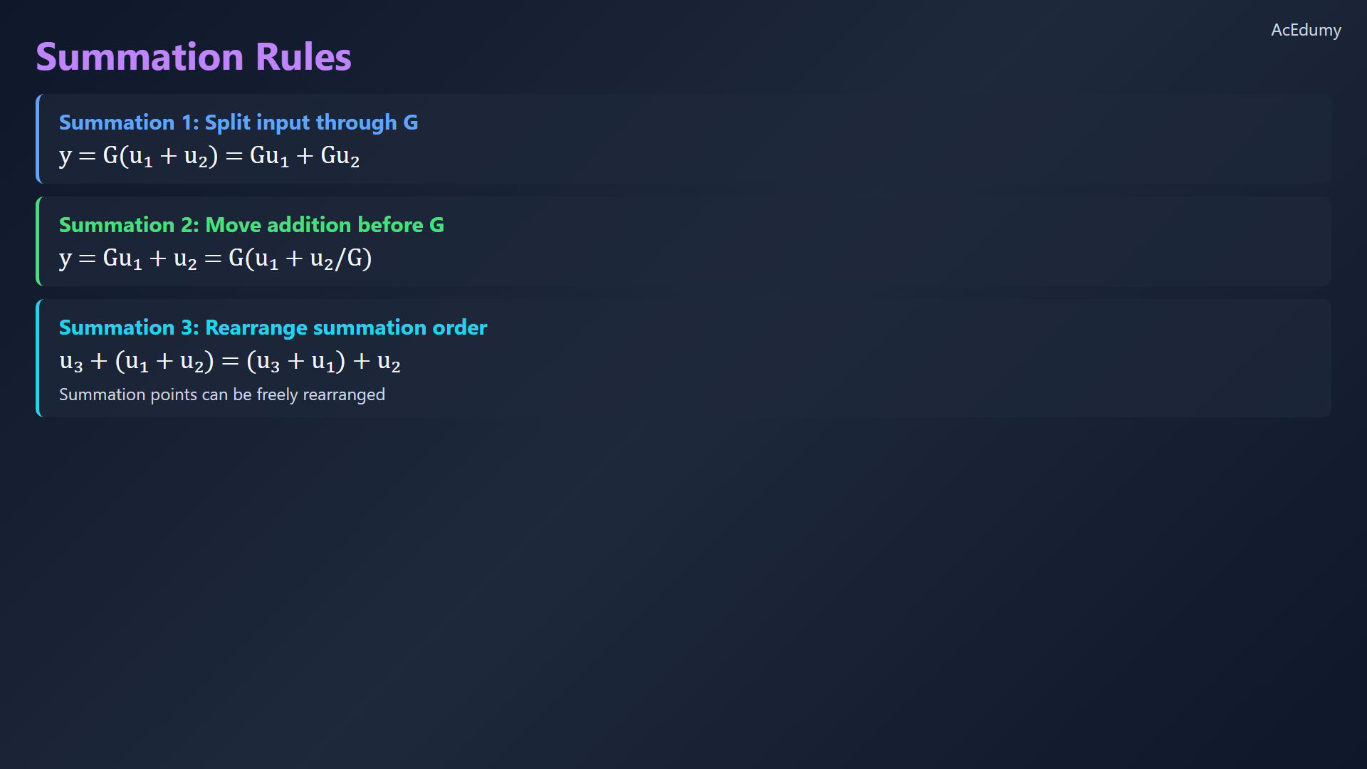
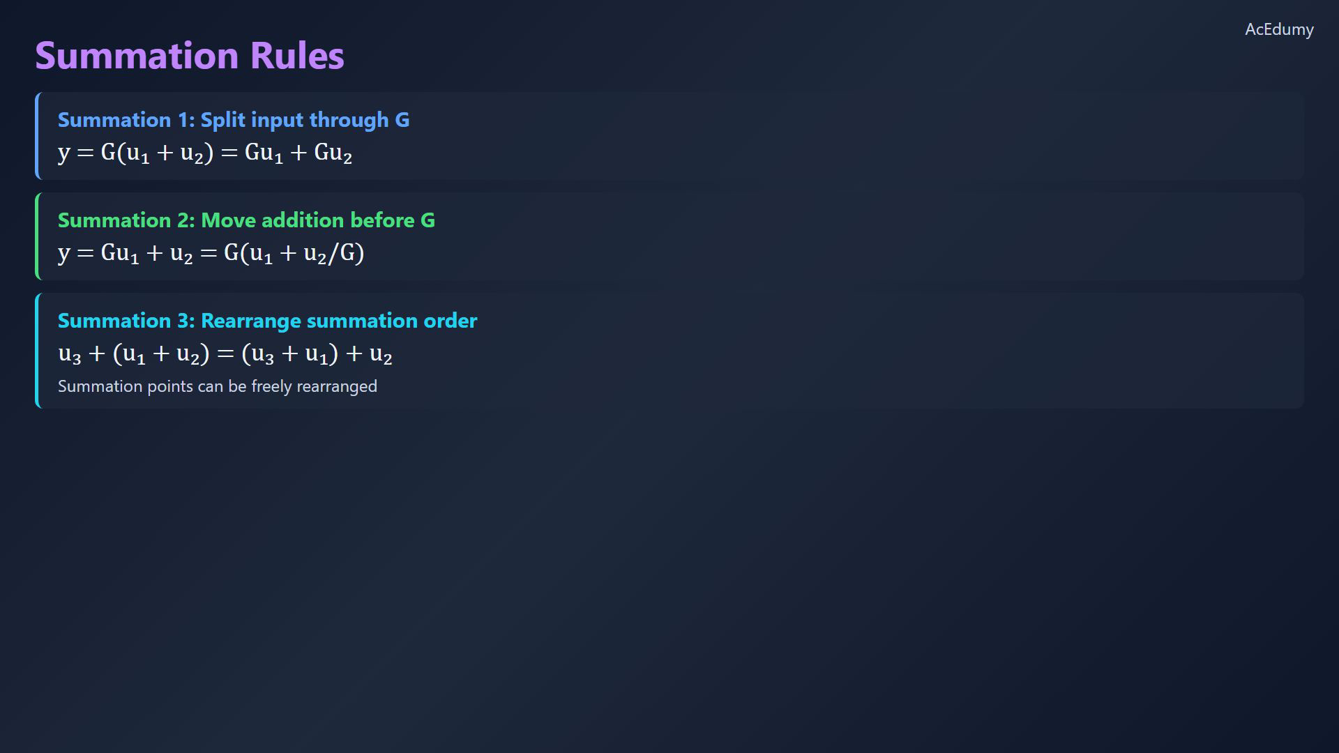
Next, three summation rules. Summation 1: if a block G receives the sum of two inputs u1 and u2, we can split it into two parallel paths, each through G. Summation 2: if a signal u2 is added after block G, we can move the addition before G by passing u2 through 1 over G. Summation 3: summation points can be freely rearranged — the order of addition doesn't matter.
4. Derive the signed feedback transfer
Use scalar zero-state LTI transfer relations. Parallel connections use the summation identity card; the full motor and outer-loop drawing use the final two-input result as an algebraic reference. The motor plots show separate 1 V voltage and 0.001 N m load steps with the other input zero. Define K as the whole fixed motor coupling c phi F.
Derive the signed feedback relation.
G₁ is the forward path; G₂ maps output into the feedback signal.
Negative-feedback input:
$\displaystyle e = u - G₂ \cdot y$
Output equation:
$\displaystyle y = G₁\left(u - G₂ \cdot y\right)$
Collect output terms:
$\displaystyle y\left(1 + G₁G₂\right) = G₁ \cdot u$
Negative feedback:
$\displaystyle G =\frac{ G₁}{1 + G₁G₂}$
Positive feedback:
$\displaystyle G =\frac{ G₁}{1 - G₁G₂}$
Narration transcript
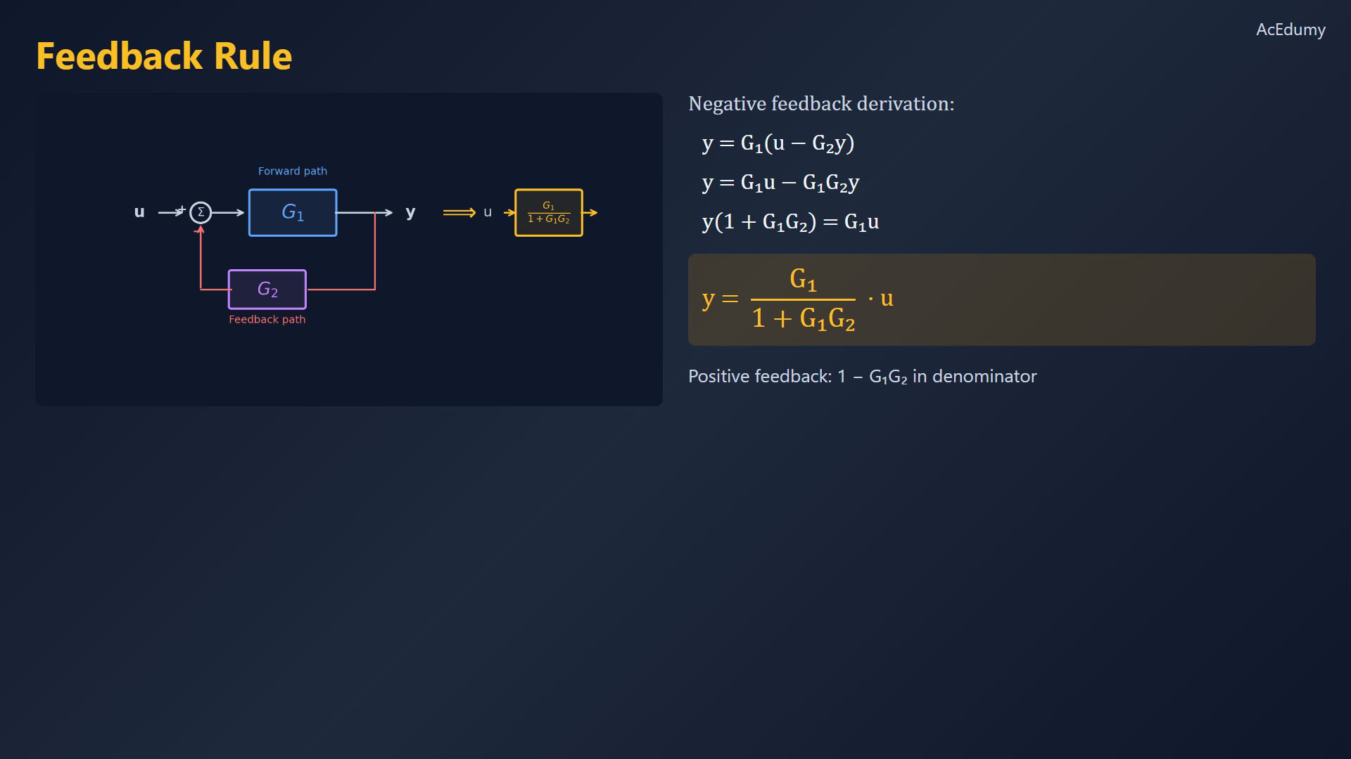
The most important rule is the feedback rule. A forward path G1 has a feedback path G2 returning from output to input. For negative feedback, the input to G1 is u minus G2 times y. So y equals G1 times the quantity u minus G2 y. Rearranging: y times 1 plus G1 G2 equals G1 u. The closed-loop transfer function is G1 divided by 1 plus G1 G2. For positive feedback, the denominator becomes 1 minus G1 G2.
5. Read the two-input motor model
Use scalar zero-state LTI transfer relations. Parallel connections use the summation identity card; the full motor and outer-loop drawing use the final two-input result as an algebraic reference. The motor plots show separate 1 V voltage and 0.001 N m load steps with the other input zero. Define K as the whole fixed motor coupling c phi F.
Use zero initial current and speed in the ideal DC motor.
Electrical balance:
$\displaystyle L_{a} \cdot i_{a}' = u - R_{a} \cdot i_{a} - K\omega$
Whole fixed torque/back-EMF coefficient:
$\displaystyle K = c \cdot \varphi _{F}$
Mechanical balance:
$\displaystyle J \cdot \omega ' = K \cdot i_{a} - T_{L}$
Subtract resistance voltage and back-EMF as two distinct feedback contributions.
Narration transcript
Now let's apply these rules to the DC motor from Lesson 9. The full block diagram has: input voltage u through a summation, then 1 over La s for inductance, producing armature current. Current times c phi F gives electrical torque. After subtracting load torque TL, the integrator 1 over J s gives angular velocity omega. The Ra feedback models armature resistance, and c phi F feedback models back-EMF.
6. Reduce the resistance loop
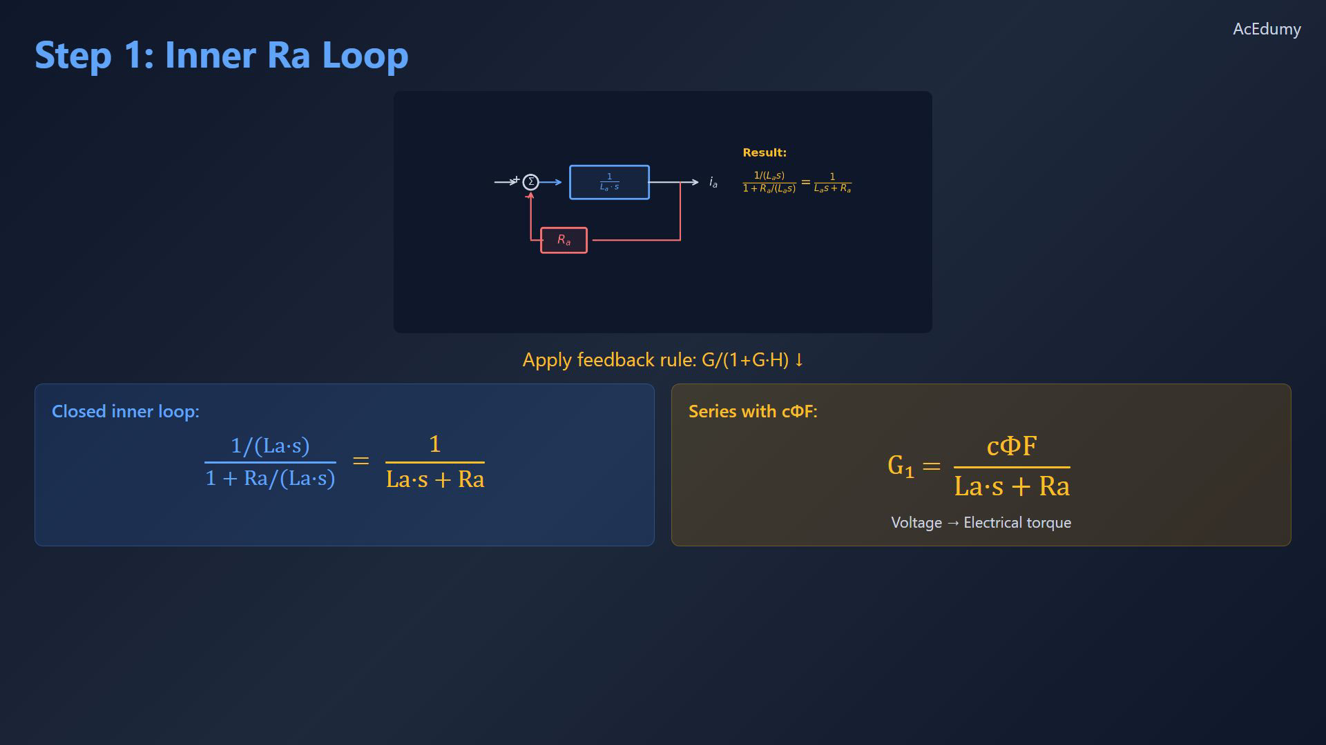
Use scalar zero-state LTI transfer relations. Parallel connections use the summation identity card; the full motor and outer-loop drawing use the final two-input result as an algebraic reference. The motor plots show separate 1 V voltage and 0.001 N m load steps with the other input zero. Define K as the whole fixed motor coupling c phi F.
Reduce the negative resistance feedback around the electrical integrator.
Forward path is the reciprocal of La times s; feedback gain is Ra.
Reduced electrical path:
$\displaystyle H =\frac{ 1}{L_{a} \cdot s + R_{a}}$
Series with the whole coupling coefficient:
$\displaystyle G₁ =\frac{ K}{L_{a} \cdot s + R_{a}}$
Before outer reduction, this path acts on the residual voltage after back-EMF.
Narration transcript
Step one: simplify the inner Ra feedback loop. The forward path has gain 1 over La s, and the feedback gain is Ra. Applying the feedback rule: the closed-loop becomes 1 over La s plus Ra. Combining this in series with c phi F, we get G1 equals c phi F divided by La s plus Ra. This represents the simplified path from voltage to electrical torque.
7. Reduce the back-EMF loop
Use scalar zero-state LTI transfer relations. Parallel connections use the summation identity card; the full motor and outer-loop drawing use the final two-input result as an algebraic reference. The motor plots show separate 1 V voltage and 0.001 N m load steps with the other input zero. Define K as the whole fixed motor coupling c phi F.
Reduce the outer back-EMF loop.
Retain the load subtraction between G₁ and the resulting G₂.
Feedback-path gain:
$\displaystyle H =\frac{ K^{2}}{L_{a} \cdot s + R_{a}}$
Reduced torque-to-speed block:
$\displaystyle G₂ =\frac{L_{a} \cdot s + R_{a}}{J \cdot s \cdot \left(L_{a} \cdot s + R_{a}\right) + K^{2}}$
Narration transcript
Step two: simplify the outer feedback loop. We rearrange using the summation rule so that the TL disturbance enters after the feedback is resolved. The forward path is 1 over J s, and the loop gain involves c phi F squared over La s plus Ra. Applying the feedback rule gives G2 equals 1 over J s divided by 1 plus c phi F squared over J s times La s plus Ra.
8. Separate voltage and load channels
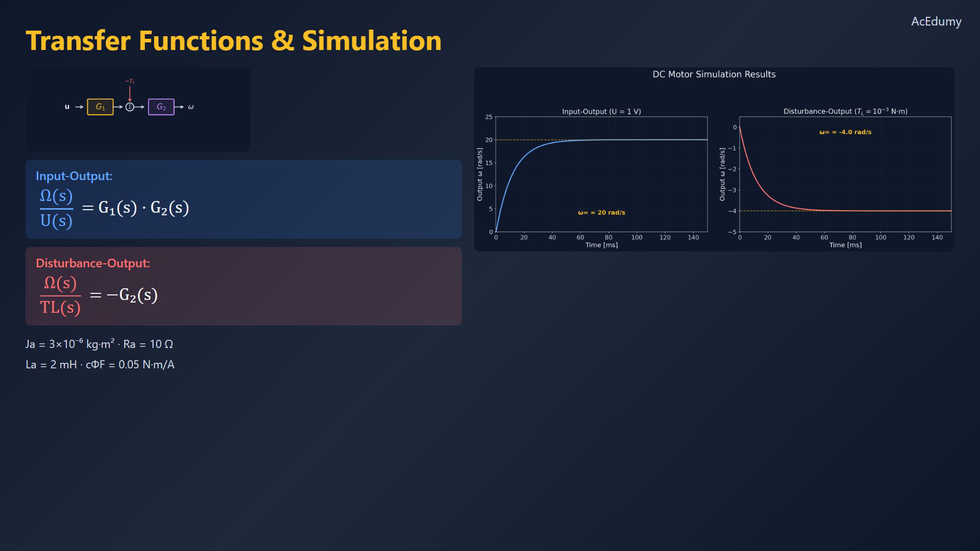
Use scalar zero-state LTI transfer relations. Parallel connections use the summation identity card; the full motor and outer-loop drawing use the final two-input result as an algebraic reference. The motor plots show separate 1 V voltage and 0.001 N m load steps with the other input zero. Define K as the whole fixed motor coupling c phi F.
Two-input result:
$\displaystyle \Omega = G₂\left(G₁ \cdot U - T_{L}\right)$
Separate the voltage and opposing-load channels with the other input zero.
With load zero:
$\displaystyle \frac{\Omega }{U }= G₁ \cdot G₂$
With voltage zero:
$\displaystyle \frac{\Omega }{T_{L} }= -G₂$
The displayed 1 V voltage step approaches 20 rad/s with load zero.
The separate 0.001 N m load step approaches −4 rad/s with voltage zero.
Approximately 50 ms describes a tolerance-based approach for these parameters.
Narration transcript
The final simplified system is elegant: voltage u passes through G1, load torque TL is subtracted, and G2 produces angular velocity omega. This gives us two clean transfer functions. Input-output: omega over U equals G1 times G2. Disturbance-output: omega over TL equals negative G2. Using typical DC motor parameters, the step response shows omega rising to about 20 radians per second. The disturbance response shows a drop of about 4 radians per second from a small torque load. Both settle within about 50 milliseconds.
9. Review the equivalent transfer model
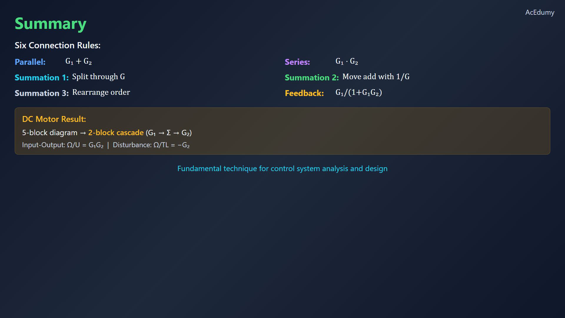
Use scalar zero-state LTI transfer relations. Parallel connections use the summation identity card; the full motor and outer-loop drawing use the final two-input result as an algebraic reference. The motor plots show separate 1 V voltage and 0.001 N m load steps with the other input zero. Define K as the whole fixed motor coupling c phi F.
Six rules, including negative feedback:
$\displaystyle G =\frac{ G₁}{1 + G₁G₂}$
The motor becomes two blocks with a load subtraction between them.
Keep voltage and disturbance channels separate before combining their responses.
Narration transcript
To summarize: six connection rules form our simplification toolkit — parallel, series, three summation rules, and the crucial feedback rule G1 over 1 plus G1 G2. We reduced the DC motor from a complex five-block diagram to a clean two-block cascade. This separation of input-output and disturbance-output behavior is fundamental to control system design.