Control Theory · Derive and Linearize a Conical Funnel Model

#33 Use the changing water-surface area, retain normalization and derive the stable local deviation model

Connect cone geometry and flow balance to equilibrium, local sensitivities and the decay time.

Question

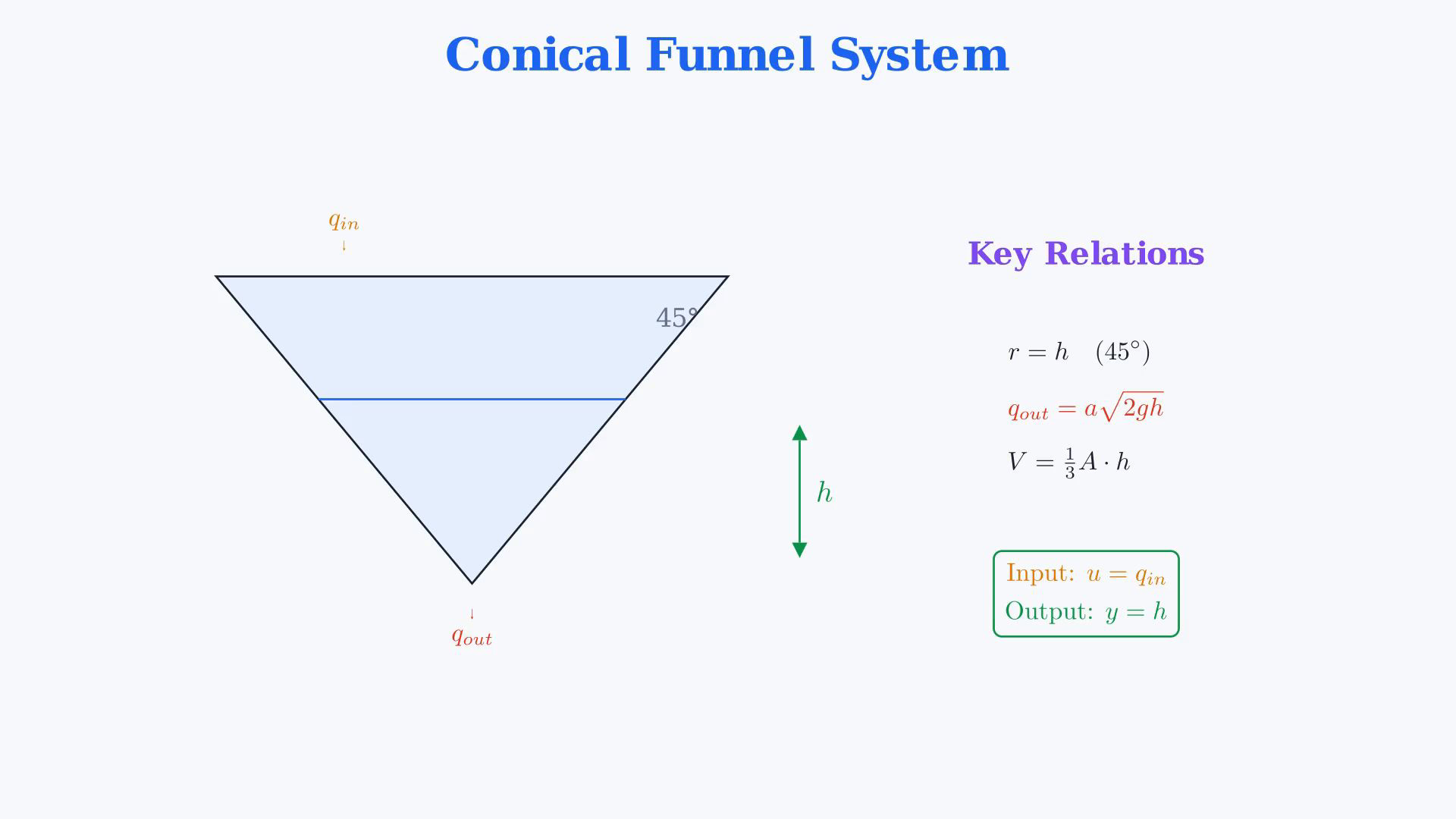
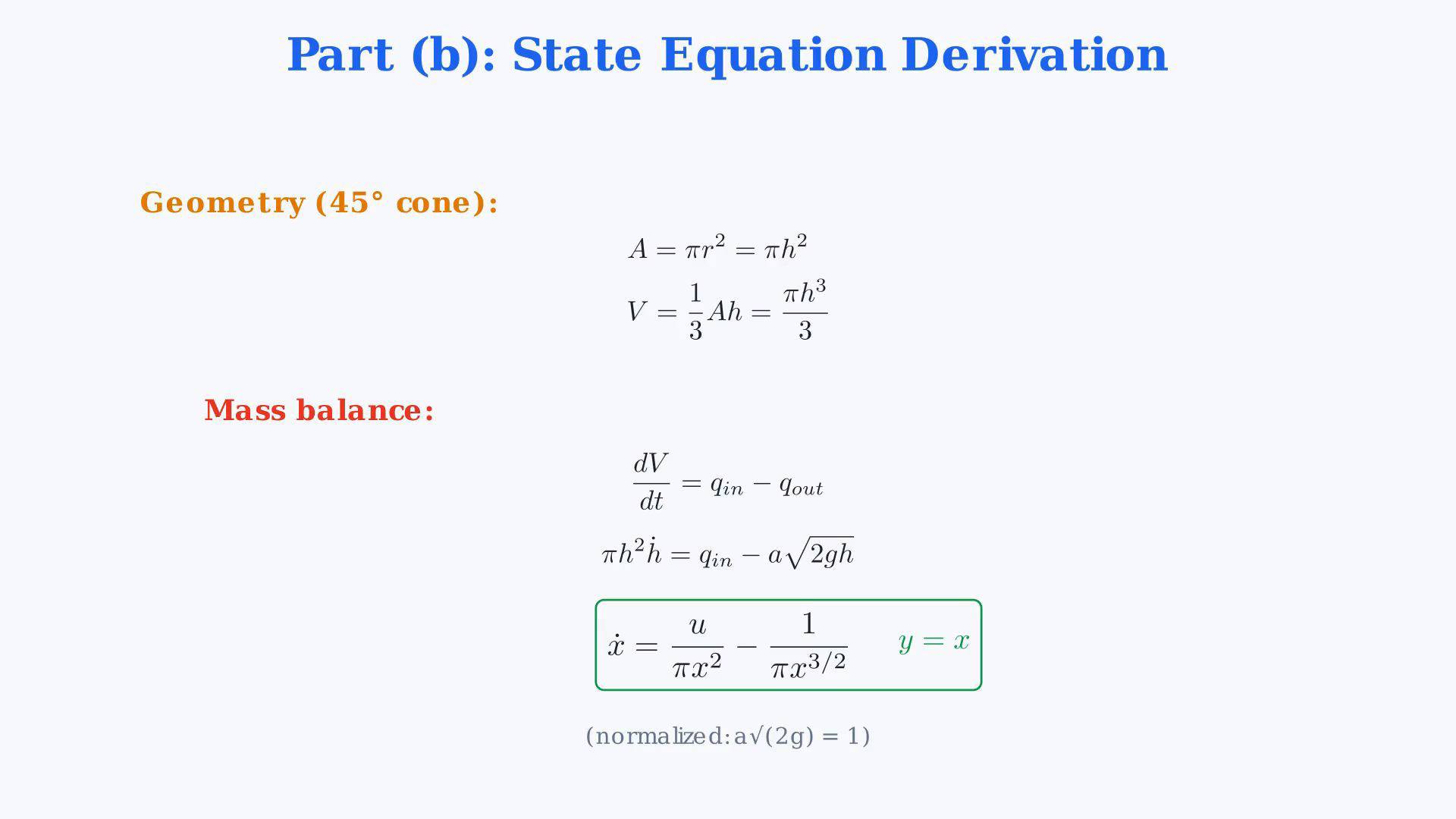
Whole existing final-video frame showing the cone geometry, nonlinear volume balance, equilibrium, partial derivatives or local deviation model. — The cone has a stated 45-degree half angle. Water-surface area varies with height; the small outlet area is constant. Numerical coefficients and the time constant use the stated normalized model.

Model the given conical funnel with an ideal small outlet at its bottom. The cone has a stated 45-degree half angle measured from its vertical axis, so its full opening angle is90 degrees and the water-surface radius is r=h. The original picture is a schematic, not a drawing from which to measure the angle or height in pixels. The state is water height h measured upward from the outlet, the controllable inflow is q_in, and the measured output is h. Assume constant fluid density, a fixed positive outlet area a_o, positive gravitational acceleration g, an ideal quasi-steady Torricelli outflow with losses neglected, and positive water height within the cone. The equations do not describe an empty outlet, overflow or arbitrary negative inflow. Distinguish the variable horizontal water-surface area A(h)=pi h² from the fixed small outlet area. The source calls the outlet area a; this notebook writes a_o when disambiguation is needed because the later scalar state-space coefficient also uses a. These are different quantities, not equal physical parameters. The water volume is V(h)=A(h)h/3=pi h³/3. Since A depends on h, differentiating V gives dV/dt=pi h² h'. It is incorrect to hold A constant and use only A h'/3. Constant density lets the mass balance reduce to the volume-flow balance dV/dt=q_in-q_out, with q_out=a_o sqrt(2gh). Consequently h'=q_in/(pi h²)-a_o sqrt(2g)/(pi h^(3/2)) for h>0. Write k=a_o sqrt(2g)>0, so the second term is -k/(pi h^(3/2)). The factor k has units length^(5/2)/time in a dimensional model. The source explicitly adopts the normalized numerical coefficient k=1 in consistent chosen coordinates and time units. With x=h,u=q_in,y=x in those coordinates, the normalized state function is f(x,u)=u/(pi x²)-1/(pi x^(3/2)). Do not silently discard k for arbitrary physical outlet areas, gravity or units; the normalization is an assumption of this worked example. At the specified x_sp=1, equilibrium with constant input requires f(1,u_sp)=0. Thus u_sp/pi-1/pi=0 and u_sp=1. The output baseline is y_sp=1. Define Delta x=x-1, Delta u=u-1 and Delta y=y-1. Differentiate the nonlinear maps before substituting the operating point. Holding u fixed, f_x=-2u/(pi x³)+3/(2pi x^(5/2)); the positive second derivative term comes from differentiating the negative power term. At(1,1), a_lin=-2/pi+3/(2pi)=(-4+3)/(2pi)=-1/(2pi). Holding x fixed, f_u=1/(pi x²), so b=1/pi. Since y=g(x,u)=x, c=g_x=1 and d=g_u=0. The source's a in its final a,b,c,d model denotes a_lin, not the outlet area a_o. In the notebook a_1(x,u) and a_2(x,u) label the two contributions to f_x; they add to the state partial and are not additional states or outlet areas. Keep the full denominators pi x^(3/2),2pi x^(5/2) and2pi grouped. The first-order local deviation model is (Delta x)'=-Delta x/(2pi)+Delta u/pi and Delta y=Delta x. Its coefficients are a_lin approximately -0.159 and b approximately0.318 in the stated normalized coordinates. These are approximate decimal values; retain their exact pi forms in calculation. The output has no direct input feedthrough, although an input change subsequently changes the water height. Restore y=1+Delta y for the absolute output. The deviation model is a local approximation of a smooth nonlinear system for x>0, not a replacement valid at the singular empty state x=0. With u held at1, the negative scalar state coefficient establishes local asymptotic stability at this positive-height equilibrium. A height slightly above1 has greater outflow than the fixed inflow and falls; a height slightly below1 has smaller outflow and rises. This conclusion is local under the stated model assumptions, not a claim about all heights, actuator constraints or a full finite funnel. The linearized free perturbation is Delta x(t)=Delta x(0)exp(-t/(2pi)). Its time constant is2pi in the chosen model time units. The source's approximately6.3 seconds applies when those units are seconds and the normalized numerical coefficient is1 in the corresponding height and flow coordinates. If time itself was nondimensionalized by a physical scale T0, the physical time constant is2pi T0 instead. No universal6.3-second time constant is implied for every funnel. As a dimensional check before imposing the source normalization, at any positive equilibrium h0 the inflow is q0=k sqrt(h0). The physical local coefficients are a_lin=-k/(2pi h0^(5/2)) and b=1/(pi h0²), giving tau=2pi h0^(5/2)/k. They reduce to the source coefficients for k=h0=1 in its chosen units. In the normalized model the equilibrium relation is h_eq=u² for positive inflow, whose local slope at u=1 is2. The zero-initial-deviation local transfer function from Delta u to Delta y is2/(1+2pi s), with DC gain2; this agrees with the equilibrium slope. It does not assert that the nonlinear equilibrium relation is globally linear.

Written solution and narration transcript(shows the full solution)

Below are all the lines written in the notebook together with the full narration transcript.

1. Read the cone geometry and flow signals
The cone has a stated 45-degree half angle. Water-surface area varies with height; the small outlet area is constant. Numerical coefficients and the time constant use the stated normalized model.
Read the funnel problem.
The vessel is an inverted cone.
The inlet flow enters at the top; the outlet flow leaves through a small bottom opening.
State and measured output:
$\displaystyle x = h; y = h$
Given 45-degree half angle:
$\displaystyle r = h$
Ideal outflow with fixed outlet area:
$\displaystyle q_{\mathrm{out}} = a_{o}\cdot \sqrt{2\cdot g\cdot h}$
Identify the controllable input and measured output.
Controllable input:
$\displaystyle u = q_{\mathrm{in}}$
Measured output:
$\displaystyle y = h$
Narration transcript
Here is the problem. We have a conical funnel, like an inverted cone. Water flows in from the top with flow rate q in, and flows out through a small opening at the bottom with flow rate q out. The height of the water level is h, measured from the bottom opening. The cone has a 45 degree half angle, which means the radius at any height equals the height itself: r equals h. The outflow depends on the opening area a and the water level: q out equals a times the square root of 2 g h. Part a asks: what are the input and output signals? The input is q in, the flow we can control. The output is h, the water level we want to observe.
2. Derive the volume balance and normalized model
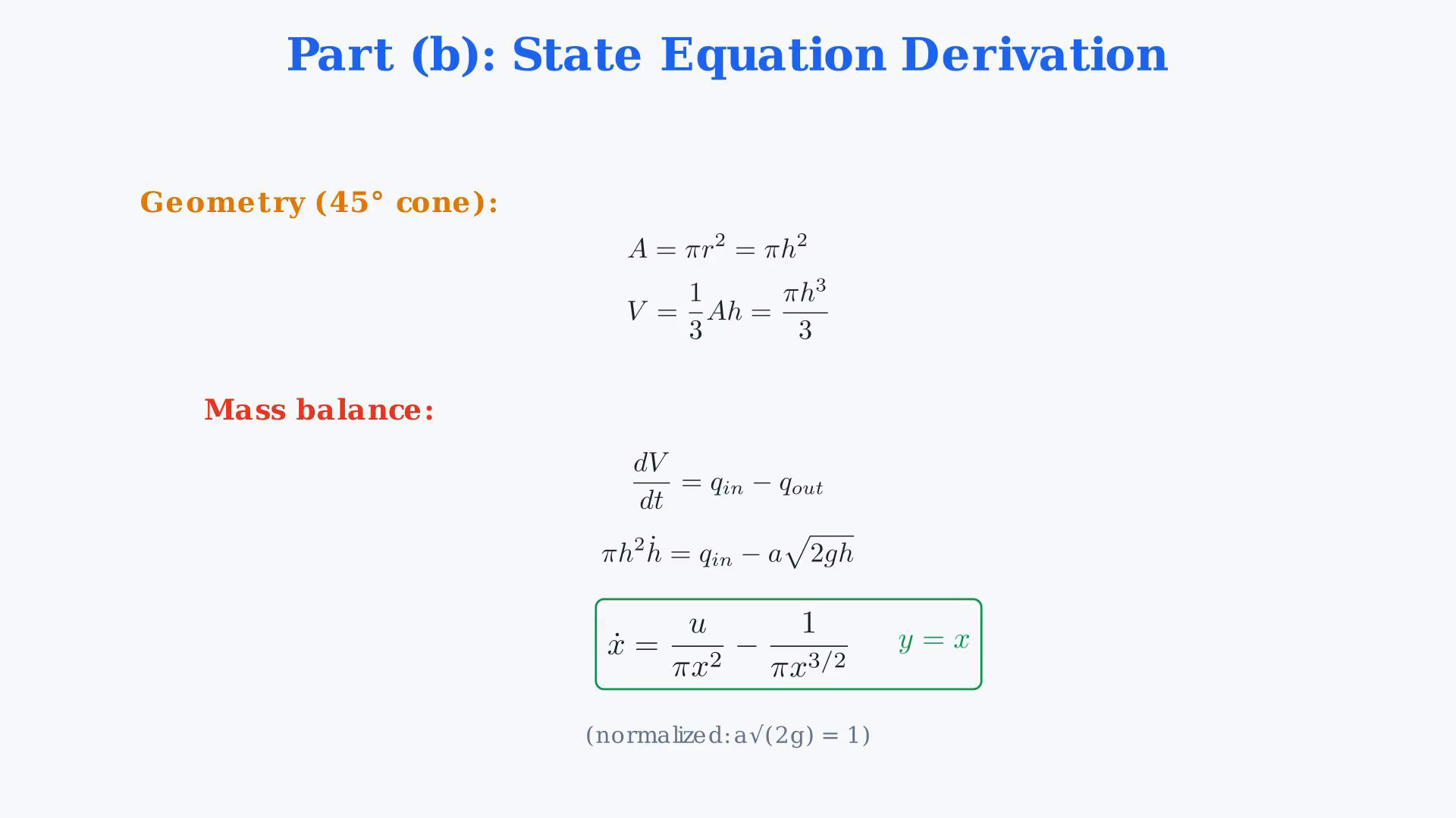
The cone has a stated 45-degree half angle. Water-surface area varies with height; the small outlet area is constant. Numerical coefficients and the time constant use the stated normalized model.
Derive the state equation from geometry and flow balance.
The stated half angle gives:
$\displaystyle r = h$
Variable water-surface area:
$\displaystyle A\left(h\right) = \pi \cdot r^{2} = \pi \cdot h^{2}$
Cone water volume:
$\displaystyle V\left(h\right) = A\left(h\right)\cdot \frac{h}{3 }= \pi \cdot \frac{h^{3}}{3}$
For constant density, the volume rate equals inflow minus outflow.
Volume balance:
$\displaystyle V' = q_{\mathrm{in}}-q_{\mathrm{out}}$
Differentiate the changing volume:
$\displaystyle V' = \pi \cdot h^{2}\cdot h'$
Substitute the ideal outflow:
$\displaystyle \pi \cdot h^{2}\cdot h' = q_{\mathrm{in}}-a_{o}\cdot \sqrt{2\cdot g\cdot h}$
Positive-height model:
$\displaystyle h' =\frac{ q_{\mathrm{in}}}{\pi \cdot h^{2}}-a_{o}\cdot \frac{\sqrt{2\cdot g}}{\pi \cdot h^{3/2}}$
Normalized coefficient and signals:
$\displaystyle a_{o}\cdot \sqrt{2\cdot g} = 1; x = h; u = q_{\mathrm{in}}; x' =\frac{ u}{\pi \cdot x^{2}}-\frac{1}{\pi \cdot x^{3/2}}$
Output equation:
$\displaystyle y = x$
Narration transcript
Part b: let us derive the state equations. Because of the 45 degree angle, the radius at height h equals h. The water surface area is A equals pi r squared, which is pi h squared. The water volume is V equals one third A h, which gives pi h cubed divided by 3. Now apply mass balance: the rate of change of volume equals inflow minus outflow. d V d t equals q in minus q out. Taking the derivative of V: d V d t equals pi h squared times h dot. So pi h squared times h dot equals q in minus a times the square root of 2 g h. Solving for h dot: h dot equals q in divided by pi h squared, minus a times the square root of 2 g, divided by pi h to the power 3 over 2. Using the normalized version where a times the square root of 2 g equals 1, with state x equals h and input u equals q in, we get: x dot equals u divided by pi x squared, minus 1 divided by pi x to the power 3 over 2. And y equals x.
3. Find the equilibrium inflow
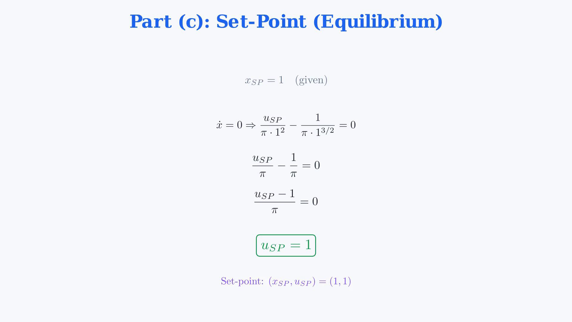
The cone has a stated 45-degree half angle. Water-surface area varies with height; the small outlet area is constant. Numerical coefficients and the time constant use the stated normalized model.
Specified operating height:
$\displaystyle x_{\mathrm{sp}} = 1$
Constant equilibrium condition:
$\displaystyle x' = 0$
Substitute the operating height:
$\displaystyle \frac{u_{\mathrm{sp}}}{\pi \cdot 1^{2}}-\frac{1}{\pi \cdot 1^{3/2}}= 0$
Simplify the balance:
$\displaystyle \frac{u_{\mathrm{sp}}}{\pi }-\frac{1}{\pi }= 0$
Equilibrium inflow:
$\displaystyle u_{\mathrm{sp}} = 1$
Operating point:
$\displaystyle x_{\mathrm{sp}} = 1; u_{\mathrm{sp}} = 1$
Narration transcript
Part c: linearize around x set-point equals 1. First, we need to find u set-point from the equilibrium condition x dot equals zero. Setting x dot to zero: u set-point divided by pi times 1 squared, minus 1 divided by pi times 1 to the power 3 over 2, equals zero. This simplifies to u set-point over pi minus 1 over pi equals zero. Therefore u set-point equals 1. Our set-point is x equals 1 and u equals 1.
4. Differentiate both state terms
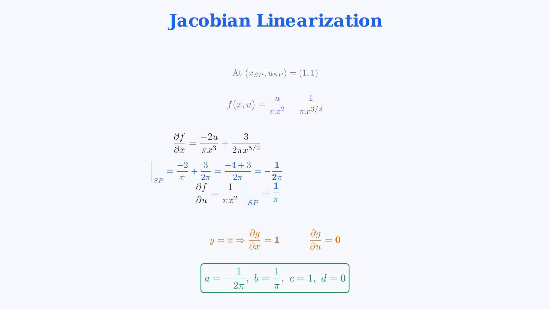
The cone has a stated 45-degree half angle. Water-surface area varies with height; the small outlet area is constant. Numerical coefficients and the time constant use the stated normalized model.
Compute the Jacobian before evaluating the operating point.
Normalized state map:
$\displaystyle f\left(x,u\right) =\frac{ u}{\pi \cdot x^{2}}-\frac{1}{\pi \cdot x^{3/2}}$
First term contribution to the state partial:
$\displaystyle a_{1}\left(x,u\right) = -2\cdot \frac{u}{\pi \cdot x^{3}}$
Second term contribution to the state partial:
$\displaystyle a_{2}\left(x,u\right) =\frac{ 3}{2\cdot \pi \cdot x^{5/2}}$
Evaluate the state partial at the operating point:
$\displaystyle a_{\mathrm{lin}} = -\frac{2}{\pi }+\frac{3}{2\cdot \pi }$
Use a common denominator:
$\displaystyle a_{\mathrm{lin}} = -\frac{4}{2\cdot \pi }+\frac{3}{2\cdot \pi }= -\frac{1}{2\cdot \pi }$
Input partial:
$\displaystyle \frac{\partial f}{\partial u }=\frac{ 1}{\pi \cdot x^{2}}$
Evaluate the input partial:
$\displaystyle b =\frac{ 1}{\pi }$
Output partials:
$\displaystyle c =\frac{ \partial g}{\partial x }= 1; d =\frac{ \partial g}{\partial u }= 0$
Narration transcript
Now compute the Jacobian. The state function is f of x, u equals u divided by pi x squared, minus 1 divided by pi x to the 3 over 2. The partial derivative of f with respect to x: from the first term, we get negative 2 u divided by pi x cubed. From the second term, we get positive 3 divided by 2 pi x to the 5 over 2. At x equals 1, u equals 1: negative 2 over pi plus 3 over 2 pi. Finding a common denominator: negative 4 over 2 pi plus 3 over 2 pi equals negative 1 over 2 pi. The partial derivative of f with respect to u equals 1 divided by pi x squared. At the set-point: 1 over pi. For the output y equals x: partial g partial x equals 1, and partial g partial u equals zero.
5. Interpret the local deviation model
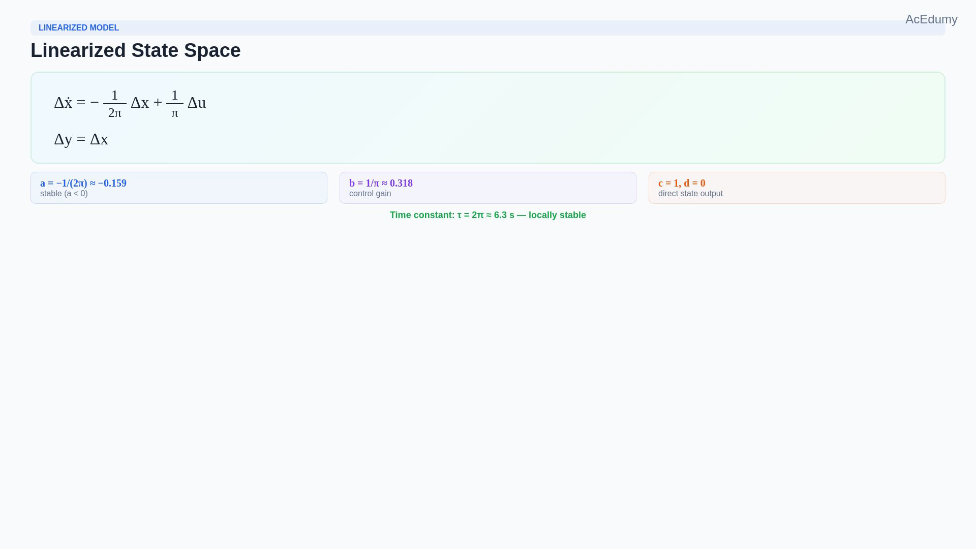
The cone has a stated 45-degree half angle. Water-surface area varies with height; the small outlet area is constant. Numerical coefficients and the time constant use the stated normalized model.
Local state deviation model:
$\displaystyle \left(\Delta x\right)' = -\frac{\Delta x}{2\cdot \pi }+\frac{\Delta u}{\pi }$
Output deviation:
$\displaystyle \Delta y = \Delta x$
State coefficient:
$\displaystyle a_{\mathrm{lin}} = -\frac{1}{2\cdot \pi }\approx -0.159$
Input coefficient:
$\displaystyle b =\frac{ 1}{\pi }\approx 0.318$
Output coefficients:
$\displaystyle c = 1; d = 0$
The negative state coefficient gives local stability with the inflow fixed at equilibrium.
A slightly higher water level increases outflow and returns toward equilibrium.
Time constant in the chosen model time units:
$\displaystyle \tau = 2\cdot \pi$
Narration transcript
Putting it all together, the linearized state space model is: delta x dot equals negative 1 over 2 pi times delta x, plus 1 over pi times delta u. delta y equals delta x. In the standard a, b, c, d form: a equals negative 1 over 2 pi, which is approximately negative 0.159. b equals 1 over pi, approximately 0.318. c equals 1 and d equals zero. Notice that a is negative, meaning the system is locally stable around this set-point. If the water level is slightly above equilibrium, the increased outflow brings it back down. The time constant is 2 pi, about 6.3 seconds.
6. Review normalization and local stability
The cone has a stated 45-degree half angle. Water-surface area varies with height; the small outlet area is constant. Numerical coefficients and the time constant use the stated normalized model.
Review the funnel analysis.
Use the stated 45-degree cone half angle.
Geometry and volume:
$\displaystyle r = h; A\left(h\right) = \pi \cdot h^{2}; V\left(h\right) = \pi \cdot \frac{h^{3}}{3}$
The nonlinear state equation contains inverse square and inverse three-halves powers of height.
The normalized equilibrium condition gives:
$\displaystyle u_{\mathrm{sp}} = 1$
At the chosen unit height and inflow:
$\displaystyle \left(\Delta x\right)' = -\frac{\Delta x}{2\cdot \pi }+\frac{\Delta u}{\pi }$
With inflow held at equilibrium, the negative local state coefficient gives local asymptotic stability.
The signal choice, nonlinear model and local linearization complete the three parts.
Narration transcript
Let us recap. We modeled a conical funnel with a 45 degree half angle. The key geometric insight: r equals h gives A equals pi h squared and V equals pi h cubed over 3. The mass balance gave us a nonlinear state equation with x to the negative 2 and x to the negative 3 over 2 terms. We found the set-point u equals 1 from the equilibrium condition. Linearizing at x equals 1, u equals 1, we got delta x dot equals negative 1 over 2 pi delta x plus 1 over pi delta u. The negative sign in a means the system is locally stable. Three parts, one complete funnel analysis, done.