#08 Control Theory #08 - Drawing Block Diagrams from RLC Circuit

Below are all the lines written in the notebook together with the full narration transcript.

1. 1. Second-order block diagram

   Corrected solution notes. The audio is the original recording and may contain errors or incomplete phrases. Where they differ, use the corrected written solution.

   Build a realization of the displayed second-order equation while preserving its input coefficient and derivative order.

   All following integral and transfer equations assume zero initial state unless stated otherwise.

   Narration transcript

   Hello everyone! Welcome to lesson eight of our control theory course. In this video, we're going to tackle something more challenging. We will draw a complete block diagram from the RLC parallel circuit differential equation. This is a second-order system, which means we'll need to handle double integrals.

2. 2. Four-step method

   Identify input u and output y; integrate consistently; isolate the output; verify the resulting diagram by recovering the starting equation.

   Narration transcript

   Before we begin, let's quickly review our four-step method. Step one: check that input and output are labeled as u and y. Step two: eliminate all derivatives by taking integrals. Step three: isolate y on one side of the equation. And step four: draw the block diagram following the equation.

3. 3. Starting equation

   y'' + y'/(RC) + y/(LC) = u/(LC)

   R, L and C are positive constants. The corrected notebook follows this displayed starting equation.

   Narration transcript

   Here's our RLC differential equation. Notice that we have a second derivative of y, which makes this a second-order system. We also have a first derivative term and a regular y term. On the right side, we have our input u.

4. 4. Input and output

   u is the forcing input in the displayed equation, and y is its output.

   Do not silently reinterpret u as its derivative or as a different physical source.

   Narration transcript

   Let's start with step one. We need to verify that our equation uses u for input and y for output. Looking at the equation, yes, we already have u as our input and y as our output. So step one is complete!

5. 5. Define integration

   Let J denote integration from time zero. Applying J twice to every term preserves the equation.

   Narration transcript

   Now comes step two, which is a bit more involved this time. We need to eliminate all derivatives by taking integrals. Since we have a second-order derivative, we'll need to take a double integral.

6. 6. Initial conditions

   $\displaystyle J²\left(y''\right)=y-y\left(0\right)-t y'\left(0\right).$

   With zero initial displacement and velocity this reduces to y. Nonzero initial conditions must be supplied as integrator states.

   Narration transcript

   Here's the key concept for second-order systems. To eliminate a second derivative, we need to integrate twice. When we apply a double integral to the second derivative of y, we get just y. The two integrals cancel out the two derivatives.

7. 7. Integrate term by term

   Under zero initial conditions: J²(y'')=y and J²(y')=J(y).

   The undifferentiated output becomes J²(y), not J(y).

   Narration transcript

   Let me show you term by term. The second derivative term becomes y after double integration. The first derivative term becomes a single integral of y, because one derivative and one integral cancel out, leaving one integral. And the regular y term becomes a double integral of y.

8. 8. Input term

   The input becomes J²(u)/(LC).

   Its coefficient remains 1/(LC), and its integration order remains two.

   Narration transcript

   For the input term on the right side, the same double integral applies. So our input u becomes a double integral of u. Now we have our equation in integral form with no derivatives!

9. 9. Isolate the output

   y = J²(u)/(LC) − J(y)/(RC) − J²(y)/(LC)

   Narration transcript

   Step three is to isolate y. We want y equals something on the right side. This is where we rearrange all the terms to get y by itself.

10. 10. Combine equal orders

    Terms may be combined only when their integration orders agree.

    J²(u)/(LC)−J²(y)/(LC)=J²(u−y)/(LC).

    Narration transcript

    Here's a useful tip from the previous lesson. When we have integrals of the same order, we can combine them inside a single integral. This makes the block diagram much easier to draw.

11. 11. First feedback term

    The first-derivative term contributes −J(y)/(RC) after isolating y.

    Narration transcript

    Let's start rearranging. I move the integral terms to the right side. First, the single integral term: one over R times the integral of y. This comes from the first derivative term.

12. 12. Second feedback term

    The output term contributes −J²(y)/(LC). Both feedback signs follow directly from moving positive terms to the right.

    Narration transcript

    Next, the double integral term: one over L times the double integral of y. I'm keeping track of the signs carefully. These terms had positive signs in the original equation, so they become negative when moved to the other side.

13. 13. Correct the combination

    A double integral of u cannot be combined as a single integral of u−y/R.

    Correct combination: y=J²((u−y)/(LC))−J(y)/(RC).

    Narration transcript

    Now I combine the input and the single integral term. They're both under a single integral, so I can write: integral of u minus one over R times y. This is much cleaner!

14. 14. Correct integral equation

    $\displaystyle Cy =\frac{ J²\left(u\right)}{L }-\frac{ J\left(y\right)}{R }-\frac{ J²\left(y\right)}{L}$

    This replaces the source's inconsistent single-integral input path.

    Narration transcript

    Here's our final equation with y isolated. Y equals one over C times the entire expression in brackets. Inside the brackets, we have: the integral of u minus one over R times y, minus one over L times the double integral of y.

15. 15. Choose a realization

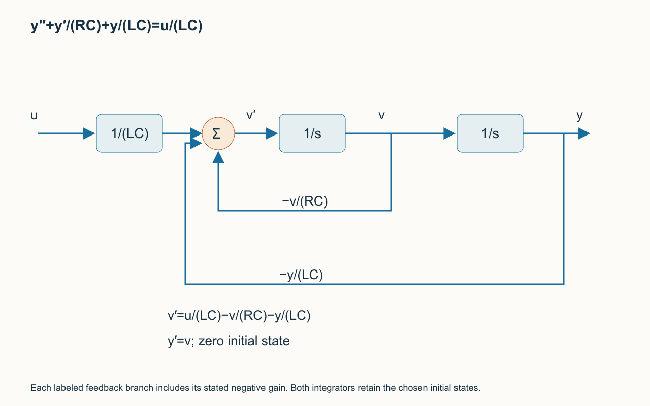
    An economical realization uses two cascaded integrators.

    Compute acceleration from u, velocity and position; integrate acceleration to velocity, then velocity to y.

    Narration transcript

    Now for the exciting part - step four, drawing the block diagram! We start with the basic structure: input u on the left, output y on the right. Then we fill in what happens in between.

16. 16. Define the state signals

    Let v=y'.

    v' = u/(LC) − v/(RC) − y/(LC)

    $\displaystyle y' = v$

    Narration transcript

    I draw the input arrow labeled u, and the output arrow labeled y. These are the two endpoints of our block diagram. Everything else connects these two points through the equation we derived.

17. 17. Position feedback

    Feed y through gain 1/(LC) to the negative input of the acceleration summing junction.

    Narration transcript

    Let's trace the first feedback path. We take y, integrate it once, multiply by one over L, then integrate again. This gives us the double integral term: one over L times double integral of y.

18. 18. Two integrators

    The first integrator maps v' to v; the second maps v to y.

    Their initial states are y'(0) and y(0).

    Narration transcript

    I draw two integrator blocks in series. The output y goes into the first integrator, giving us integral of y. Then into the second integrator, giving us double integral of y. The one over L gain block comes before or after - your choice!

19. 19. Velocity feedback

    Feed v through gain 1/(RC) to the negative input of the same acceleration junction.

    Narration transcript

    Now the second feedback path. We take y, multiply by one over R, and this connects to the summing junction along with u. This is the single integral term: one over R times y.

20. 20. Resistor coefficient

    The velocity feedback coefficient is 1/(RC). A gain changes amplitude; it does not integrate.

    Narration transcript

    I draw a gain block with one over R. The input is y, the output goes to the summing junction. This represents the term one over R times y in our equation.

21. 21. Summing junction

    Add u/(LC), subtract v/(RC), and subtract y/(LC).

    The junction output is acceleration v'.

    Narration transcript

    Here's where it gets interesting. We need summing junctions to combine our terms. One junction adds u and subtracts one over R times y. Another junction subtracts the double integral term.

22. 22. Trace the signals

    u → gain 1/(LC) → acceleration sum → integrator → v → integrator → y.

    Return both signed feedback signals to the acceleration sum.

    Narration transcript

    I draw the circular summing junction. The plus sign for u, minus sign for the one over R times y term. The output of this junction goes into an integrator. Then another summing junction for the double integral term.

23. 23. Final output

    The second integrator output is y. No additional output gain is required for this chosen realization.

    Narration transcript

    After the summing junctions, we multiply by one over C. This gives us y! I draw the one over C gain block, and its output is our final output y. The block diagram is complete!

24. 24. Verify the complete diagram

    Substituting v=y' into the summing equation recovers y''+y'/(RC)+y/(LC)=u/(LC).

    This is the essential check on every block-diagram rearrangement.

    Narration transcript

    Look at our finished block diagram! We have two feedback paths - one through one over R with a single integral, and one through one over L with a double integral. Both paths use negative feedback. The final multiplication by one over C gives us y.

25. 25. Equivalent drawings

    Different layouts may be equivalent if they preserve the equations and initial-state mapping.

    Constant gains may be regrouped consistently; changing an integration order changes the system.

    Narration transcript

    Remember, there are multiple ways to draw this diagram. You could place the gain blocks in different positions, or arrange the summing junctions differently. As long as the mathematics is correct, the diagram is valid!

26. 26. Transfer-function check

    Y/U = 1/(LCs²+(L/R)s+1)

    This is the zero-state transfer function of the starting equation. It differs from a numerator proportional to s.

    Narration transcript

    Let's summarize what we learned. For second-order systems like RLC circuits, we need double integrals. This creates two feedback paths in our block diagram. The four-step method works perfectly for these more complex systems too!

27. 27. Review

    

    Preserve every coefficient, integration order and feedback sign.

    The corrected two-integrator realization implements the displayed equation throughout.

    Narration transcript

    That concludes lesson eight! We've successfully drawn a block diagram from a second-order RLC differential equation. In the next lesson, we'll explore even more advanced topics. Thank you for watching, and I'll see you in the next video. Goodbye!

Source video: Control Theory #08 - Drawing Block Diagrams from RLC Circuit (7:05)