#23 Control Theory #23 - Root Locus Basics

Below are all the lines written in the notebook together with the full narration transcript.

1. 1. Root-locus concept

   Corrected solution notes. The audio is the original recording and may contain errors or incomplete phrases. Where they differ, use the corrected written solution.

   For a real rational negative-feedback loop, the root locus traces closed-loop roots as nonnegative gain K varies.

   Specify the feedback sign and separate fixed plant factors from K.

   Narration transcript

   So far we have analyzed stability for a fixed system. But in practice, we design controllers with adjustable gain K. As K changes, the closed loop poles move in the s plane. The root locus is the plot of all possible closed loop pole locations as K varies from zero to infinity. It is one of the most powerful tools in classical control design.

2. 2. Characteristic equation

   1 + KG(s)H(s) = 0

   In unity feedback H is one. For general sensor feedback retain H. Clear denominators and check cancellations when interpreting modes.

   Narration transcript

   Consider a unity feedback system with open loop transfer function K times G of s times H of s. The closed loop characteristic equation is one plus K times G of s times H of s equals zero. The roots of this equation are the closed loop poles. As K changes, these roots trace paths in the s plane. Those paths are the root locus.

3. 3. Branch endpoints

   There are n branches counted with multiplicity for a strictly proper loop with n poles and m zeros.

   At zero gain branches begin at open-loop poles; as gain tends to infinity, m terminate at finite zeros and n−m tend to infinity.

   Narration transcript

   Rule one: the root locus has n branches, where n is the number of open loop poles. Rule two: the branches start at the open loop poles when K equals zero. Rule three: the branches end at the open loop zeros when K approaches infinity. If there are more poles than zeros, the extra branches go to infinity along asymptotes.

4. 4. Real-axis rule

   For real coefficients the locus is symmetric about the real axis.

   Under the stated negative-feedback and positive-gain convention, a real point is on the locus when the number of real poles and zeros strictly to its right is odd.

   Narration transcript

   Rule four: the root locus is symmetric about the real axis, because complex poles always come in conjugate pairs. Rule five: a point on the real axis belongs to the root locus if the total number of real poles and zeros to its right is odd. This is called the real axis rule. Segments of the real axis that satisfy this condition are part of the locus.

5. 5. Asymptotes

   $\displaystyle \theta q =\frac{ \left(2q+1\right)\pi }{n-m}$

   The centroid is the sum of poles minus the sum of zeros, divided by n−m. Use q from zero through n−m−1.

   Narration transcript

   Rule six: when the number of poles exceeds the number of zeros, the extra branches approach infinity along straight line asymptotes. The angles of these asymptotes are given by two q plus one times one hundred eighty degrees, divided by n minus m, where q takes values zero, one, two, and so on. The asymptotes all radiate from a single point on the real axis called the centroid. The centroid is the sum of the pole locations minus the sum of the zero locations, divided by n minus m.

6. 6. Two-pole example

   For G(s)=1/(s(s+3)), the characteristic polynomial is s²+3s+K.

   The real segment is between −3 and zero; centroid and breakaway point are −1.5. The asymptotes are vertical.

   Narration transcript

   Let us plot the root locus for a simple example. G of s equals one over s times s plus three. There are two poles at s equals zero and s equals negative three. No finite zeros. Two branches start at the two poles. The real axis segment between zero and negative three is on the locus. The asymptote angles are ninety degrees and two hundred seventy degrees. The centroid is at zero plus negative three divided by two, which is negative one point five. The branches break away from the real axis at negative one point five and go vertically to infinity.

7. 7. Breakaway calculation

   K(s)=−s(s+3), so the stationary point is s=−1.5 and K=2.25.

   For larger gain the roots are −1.5 ± j√(K−2.25). Candidate stationary points must satisfy the locus and gain constraints.

   Narration transcript

   The breakaway point is where two branches leave the real axis and become complex conjugate. It occurs where the gain K is at a local maximum on the real axis segment. For our example, we can find it by setting the derivative of K with respect to s equal to zero. The branches break away at s equals negative one point five, then travel vertically upward and downward along the asymptotes.

8. 8. Choose a feasible gain

   The final sentence of the source audio in this section is incomplete; the gain-selection rule is supplied here in writing.

   A desired pole must lie on the locus; then the magnitude condition determines K.

   In the two-pole example no positive gain places a pole on the imaginary axis, because the complex branches retain real part −1.5. Check feasibility before selecting a damping line.

   Narration transcript

   The root locus is not just a picture. It is a design tool. We can choose the gain K to place the closed loop poles at desired locations. For example, if we want the poles on the imaginary axis, we find the K value where the locus crosses the imaginary axis. If we want a specific damping ratio, we draw the corresponding zeta line and find where it intersects the locus. The gain at that point gives us our design.

9. 9. Three-pole example: corrected geometry

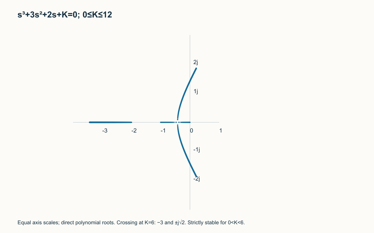
   For G(s)=1/(s(s+1)(s+2)), real-axis segments are (−∞,−2) and (−1,0).

   The centroid is −1; asymptote angles are 60°, 180° and 300°.

   The valid breakaway is −1+1/√3, approximately −0.42265. The other stationary point is not on a positive-gain segment.

   Narration transcript

   Now a slightly more complex example. G of s equals one over s times s plus one times s plus two. Three poles at zero, negative one, and negative two. No zeros. Three branches. Real axis segments: between zero and negative one, and from negative two to the left. Asymptote angles: sixty, one hundred eighty, and three hundred degrees. Centroid at negative one. Two branches break away near s equals negative zero point four two and eventually cross into the right half plane, making the system unstable for large K.

10. 10. Stability limit

    The characteristic polynomial is s³+3s²+2s+K. Its Routh first column is 1, 3, (6−K)/3, K.

    Strict stability requires 0<K<6. At K=6 the roots are −3 and ±j√2; for K>6 two roots lie in the right half-plane.

    Narration transcript

    This last point is critical. The root locus shows us the maximum gain for stability. When any branch crosses the imaginary axis into the right half plane, the system becomes unstable. The K value at that crossing is the stability limit. We can find it using the Routh Hurwitz criterion applied to the characteristic polynomial with K as a variable. This connects everything we have learned in Lecture four.

11. 11. Design summary

    

    Count branches, mark real segments, compute asymptotes and validate stationary points.

    Use the characteristic equation to check gain and stability; a schematic curve alone cannot certify a design.

    These rules provide the starting point for controller design.

    Narration transcript

    Let us summarize the root locus rules. Branches start at poles and end at zeros. The locus is symmetric about the real axis. Real axis segments follow the odd count rule. Asymptotes have specific angles and a centroid. Breakaway points occur at gain maxima on the real axis. And the locus tells us the maximum gain for stability. With this, Lecture four on stability analysis is complete. In the next lectures, we will use these tools for controller design.

Source video: Control Theory #23 - Root Locus Basics (6:03)