Control Theory · Drawing Block Diagrams from DC Motor Equations

#09 Realize the coupled current and angular-speed equations with signed gains and two integrators

Derive a two-state DC motor realization, identify the load-torque disturbance and preserve each coupling sign and initial state.

Question

Existing DC motor lesson frame showing equations or a stage in the construction of the signal-flow diagram. — The early diagram frames are partial construction stages; faded paths await their source signals. The speed-sum step uses the clean speed-equation card as an algebraic reference. The final diagram contains two integrators and three negative contributions. Compact integrals suppress their initial-value constants.

Use the ideal fixed-flux DC motor model. The input u is armature voltage, i_a is armature current, omega is angular speed, and the output y is omega. Positive load torque T_L opposes the chosen positive rotation. R_a and L_a are positive constant armature resistance and inductance; J is positive constant inertia. The product c times phi is a constant coupling coefficient, not capacitance and not the number five. With consistent SI units and this ideal fixed-flux model, the same coefficient relates speed to back EMF and current to electromagnetic torque. Write the electrical balance as applied voltage equals resistive drop plus inductive drop plus back EMF. Mechanical inertia times angular acceleration equals motor torque minus load torque. The source omits mechanical friction; do not add a friction term silently or claim that all real motors have none. Substitute the coupling relations and isolate both first time derivatives. The current rate has positive voltage contribution, negative resistive contribution and negative back-EMF contribution. The speed rate has positive motor-torque contribution and negative load-torque contribution. Every input of the current summing node has current/time units; every input of the speed summing node has angular-acceleration units. Integrate each state from the same specified initial time and retain independent initial current and speed. The compact indefinite integrals suppress constants. With lower limit zero, add i_a(0) and omega(0), respectively. A transfer block 1/s describes the zero-initial-state input/output operator; arbitrary initial states require their separate initial-value contributions. Derivatives are represented by integrators in this chosen realization; integration does not remove the dynamics or erase initial conditions. Route the voltage through gain 1/L_a; the spoken route homophone does not instruct taking a square root. Feed current through R_a/L_a to the negative electrical input and speed through c times phi divided by L_a to its other negative input. The current integrator output branches to the resistive path and to the positive mechanical path through c times phi divided by J. Feed load torque through 1/J to the negative mechanical input. The second integrator produces speed and the output. The early construction frames are intentionally partial and have faded unconnected paths before the relevant state output is drawn. The speed-sum equation card is an algebraic reference, not a completed diagram. The final diagram supplies both integrators, connected branch points, positive forward contributions and all three negative contributions. These loops are internal electrical and mechanical couplings in the plant; no separate reference, controller or sensor has been designed. Equivalent layouts must preserve equations, gains, signs, signal directions and matched initial states. Drawing the model alone supplies no tracking or regulation guarantee.

Written solution and narration transcript(shows the full solution)

Below are all the lines written in the notebook together with the full narration transcript.

1. Introduce the DC motor model
The early diagram frames are partial construction stages; faded paths await their source signals. The speed-sum step uses the clean speed-equation card as an algebraic reference. The final diagram contains two integrators and three negative contributions. Compact integrals suppress their initial-value constants.
Introduce the DC motor example.
Continue with Control Theory, Lesson 9.
Move from the RLC example to coupled motor dynamics.
Derive the block diagram directly from the motor equations.
Narration transcript
Hello everyone. Welcome to lesson 9 of our control theory course. In this lesson, we move from the RLC example to a DC motor example. Our goal is to derive a correct block diagram directly from the motor equations.
2. Identify voltage speed and load torque
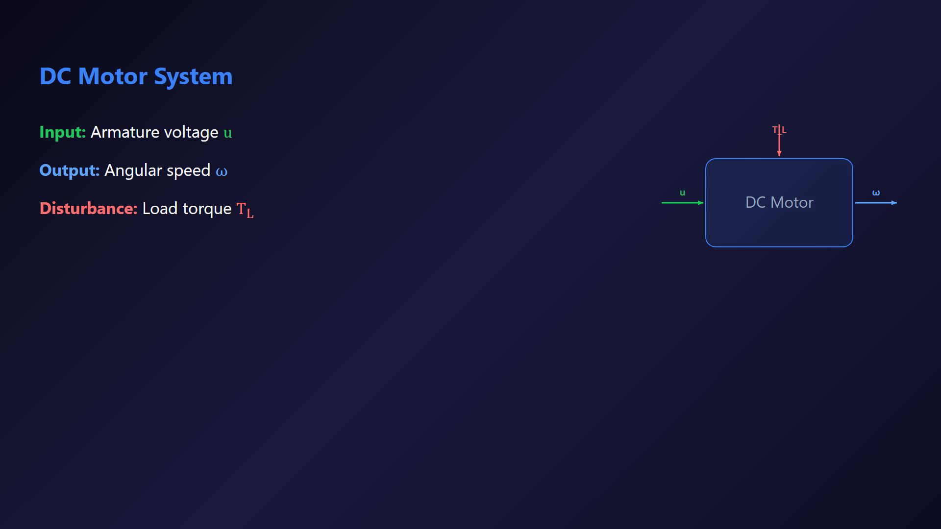
The early diagram frames are partial construction stages; faded paths await their source signals. The speed-sum step uses the clean speed-equation card as an algebraic reference. The final diagram contains two integrators and three negative contributions. Compact integrals suppress their initial-value constants.
Identify the coupled electrical and mechanical states.
Input: armature voltage u.
Output: angular speed ω.
Disturbance: opposing load torque T_L.
Narration transcript
The DC motor has electrical and mechanical parts that are coupled. Our input will be the armature voltage U. Our output will be the angular speed omega. We also include load torque as a disturbance input.
3. Write the armature voltage equation
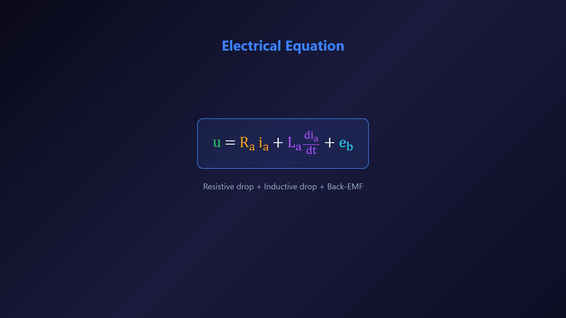
The early diagram frames are partial construction stages; faded paths await their source signals. The speed-sum step uses the clean speed-equation card as an algebraic reference. The final diagram contains two integrators and three negative contributions. Compact integrals suppress their initial-value constants.
Start with the armature electrical balance.
Applied voltage supplies resistive drop, inductive drop and back EMF.
Voltage balance:
$\displaystyle u = R_{a}\cdot i_{a} + L_{a}\cdot i_{a}'\left(t\right) + e_{b}.$
Narration transcript
Let us start with the electrical equation. Armature voltage equals resistive drop plus inductive drop plus back electromotive force. In symbols, U equals Ra times Ia plus La times dIA by dt plus EB.
4. Relate back EMF and motor torque
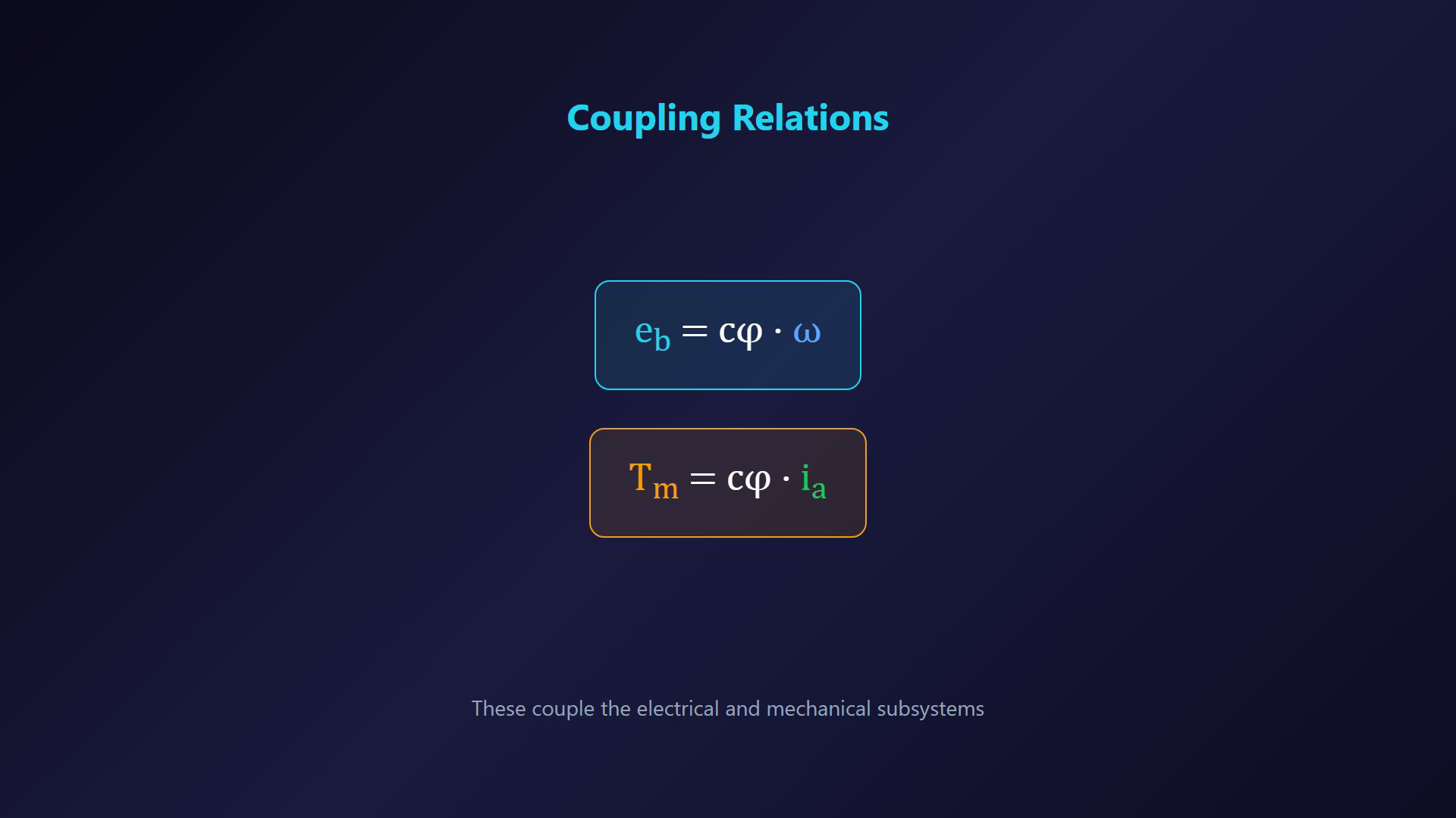
The early diagram frames are partial construction stages; faded paths await their source signals. The speed-sum step uses the clean speed-equation card as an algebraic reference. The final diagram contains two integrators and three negative contributions. Compact integrals suppress their initial-value constants.
Use the fixed-flux coupling relations with consistent units.
Back EMF:
$\displaystyle e_{b} = c\cdot \varphi \cdot \omega .$
Motor torque:
$\displaystyle T_{m} = c\cdot \varphi \cdot i_{a}.$
Narration transcript
Now we add coupling relations. Back EMF is proportional to speed, so EB equals C phi times omega. Electromagnetic torque is proportional to current, so TM equals C phi times IA.
5. Write the mechanical balance
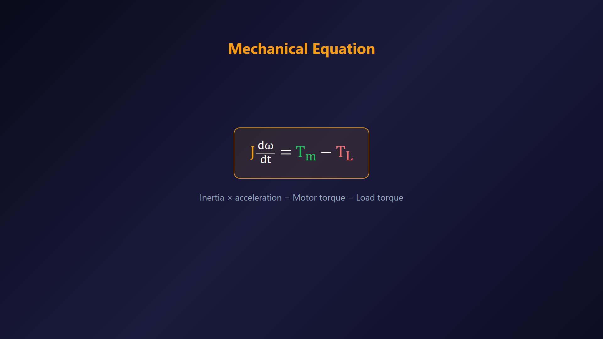
The early diagram frames are partial construction stages; faded paths await their source signals. The speed-sum step uses the clean speed-equation card as an algebraic reference. The final diagram contains two integrators and three negative contributions. Compact integrals suppress their initial-value constants.
Angular inertia times acceleration equals motor torque minus load torque.
Mechanical balance:
$\displaystyle J\cdot \omega '\left(t\right) = T_{m} - T_{L}.$
Treat positive load torque as opposing the chosen rotation.
Narration transcript
For the mechanical side, inertia times speed derivative equals motor torque minus load torque. In symbols, J times d omega by dt equals Tm minus Tl. Here, Tl is the disturbance torque.
6. Substitute the coupling relations
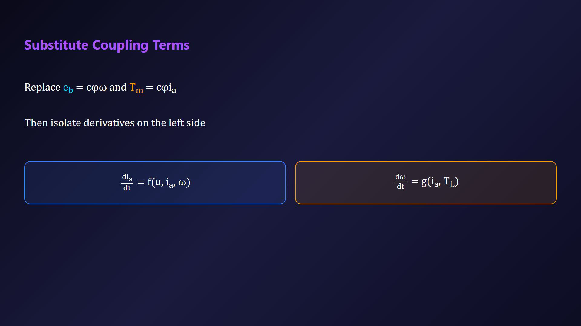
The early diagram frames are partial construction stages; faded paths await their source signals. The speed-sum step uses the clean speed-equation card as an algebraic reference. The final diagram contains two integrators and three negative contributions. Compact integrals suppress their initial-value constants.
Substitute the back-EMF and motor-torque relations.
Isolate both first time derivatives.
Obtain one state equation for current and one for speed.
Narration transcript
Substitute torque and back EMF relations into the main equations. Then, isolate derivatives on the left side. This gives us one differential equation for current and one for speed.
7. Isolate the current derivative
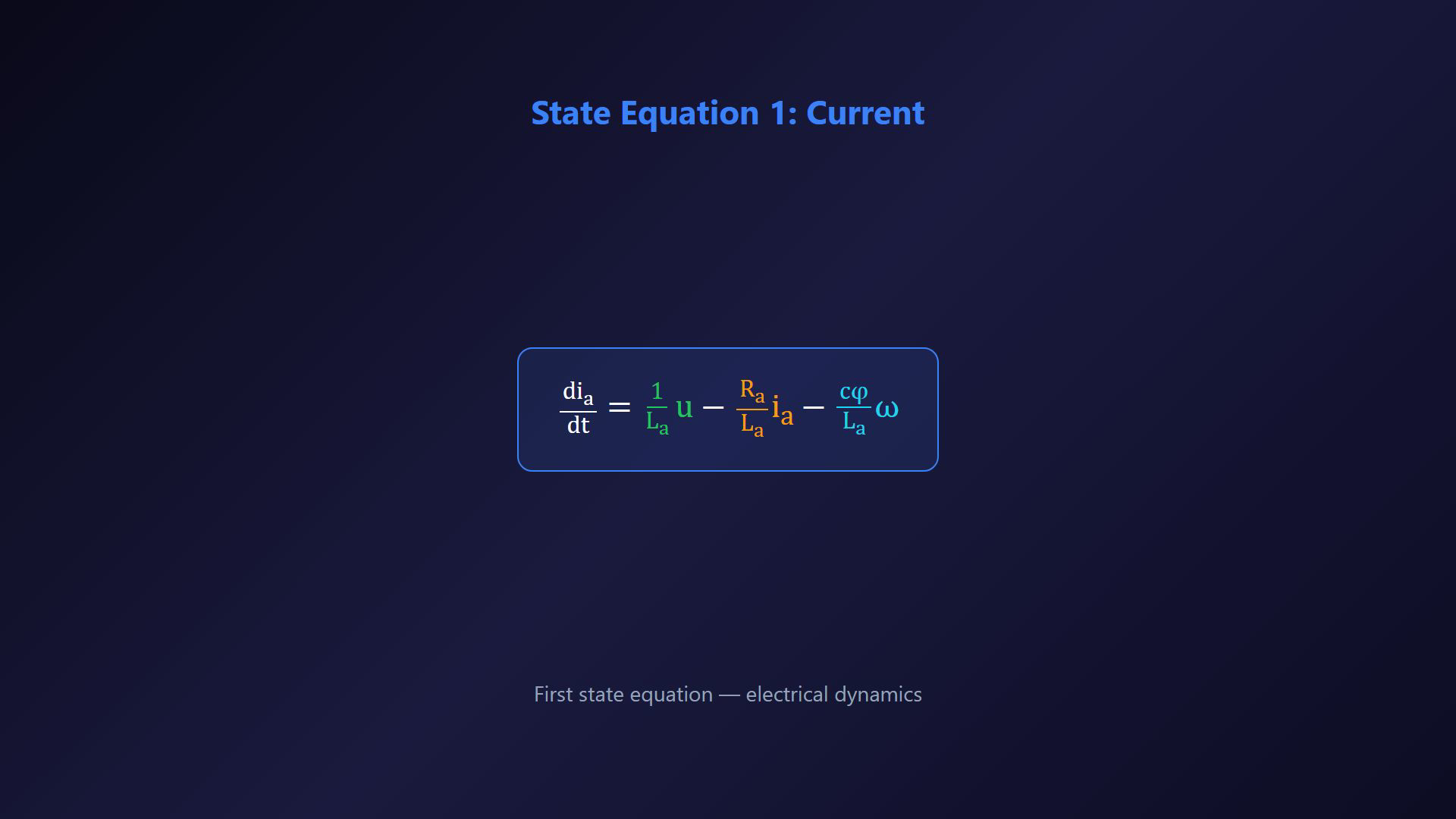
The early diagram frames are partial construction stages; faded paths await their source signals. The speed-sum step uses the clean speed-equation card as an algebraic reference. The final diagram contains two integrators and three negative contributions. Compact integrals suppress their initial-value constants.
Current state:
$\displaystyle i_{a}'\left(t\right) = \left(\frac{1}{L_{a}}\right)\cdot u - \left(\frac{R_{a}}{L_{a}}\right)\cdot i_{a} - \left(\frac{c\cdot \varphi }{L_{a}}\right)\cdot \omega .$
Preserve both negative electrical contributions.
Narration transcript
The current equation becomes dIA by dt equals 1 over LA times U minus RA over LA times IA minus Cphi over LA times omega. This is our first state equation.
8. Isolate the speed derivative
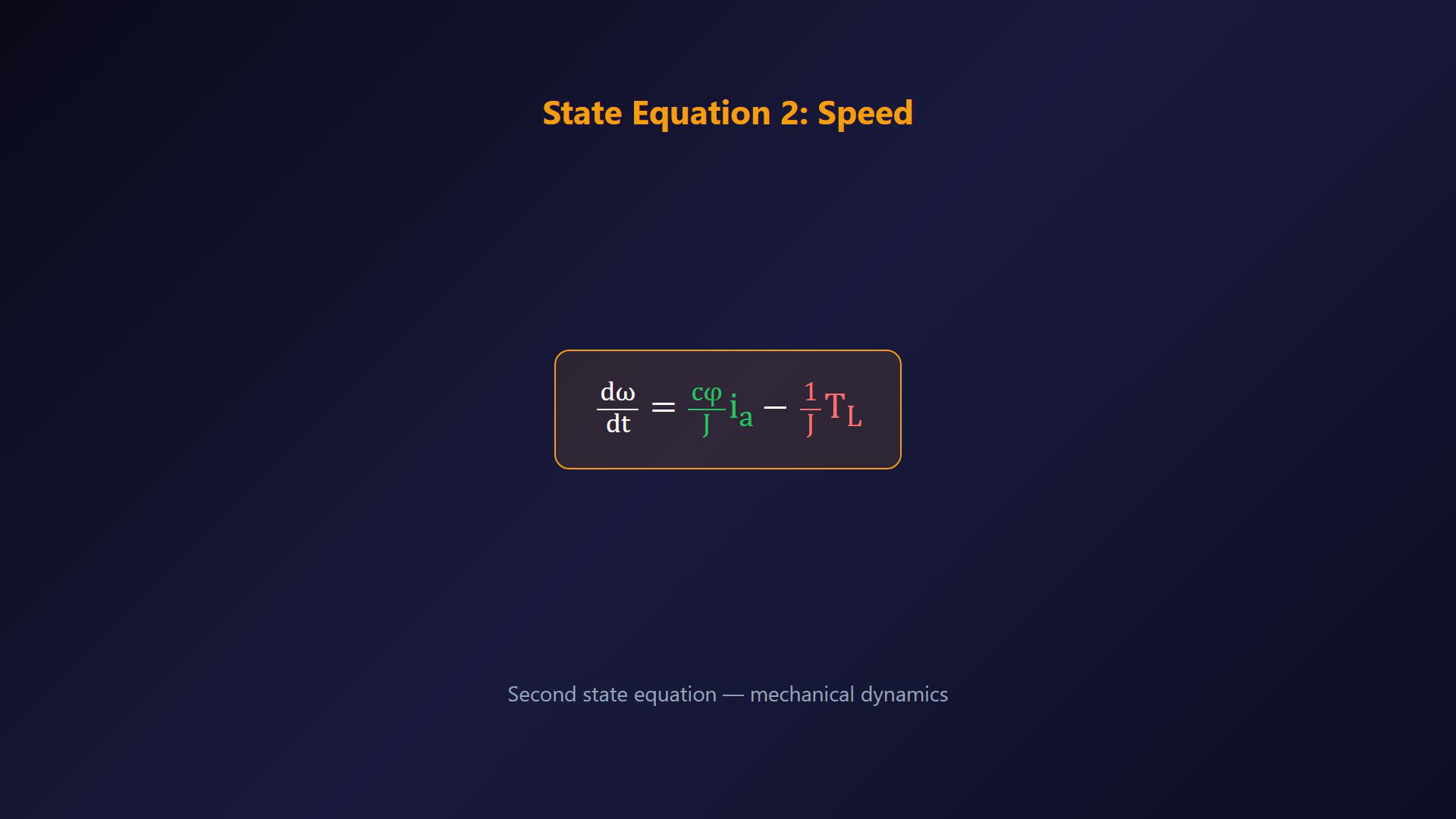
The early diagram frames are partial construction stages; faded paths await their source signals. The speed-sum step uses the clean speed-equation card as an algebraic reference. The final diagram contains two integrators and three negative contributions. Compact integrals suppress their initial-value constants.
Speed state:
$\displaystyle \omega '\left(t\right) = \left(\frac{c\cdot \varphi }{J}\right)\cdot i_{a} - \left(\frac{1}{J}\right)\cdot T_{L}.$
Preserve the opposing load-torque sign.
Narration transcript
The speed equation becomes d omega by dt equals Cphi over J times IA minus 1 over J times TL. This is our second state equation.
9. Convert both states to integral form
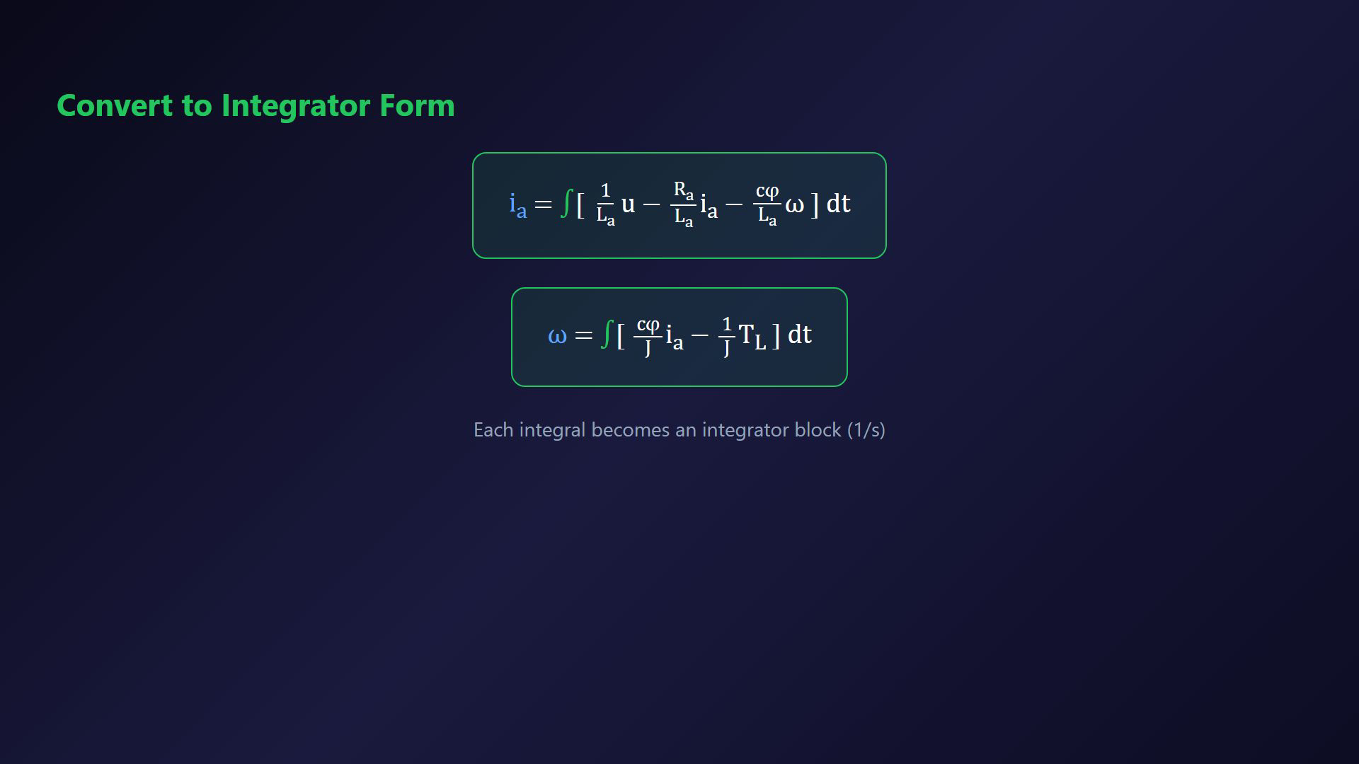
The early diagram frames are partial construction stages; faded paths await their source signals. The speed-sum step uses the clean speed-equation card as an algebraic reference. The final diagram contains two integrators and three negative contributions. Compact integrals suppress their initial-value constants.
Realize each state derivative using an integrator.
Integrate each bracket and retain its own initial current or speed.
Narration transcript
For block diagram drawing, we convert derivatives into integrator form. Integrating both equations gives Ia equals integral of the first bracket and omega equals integral of the second bracket.
10. Check the drawing method
The early diagram frames are partial construction stages; faded paths await their source signals. The speed-sum step uses the clean speed-equation card as an algebraic reference. The final diagram contains two integrators and three negative contributions. Compact integrals suppress their initial-value constants.
Check the four-step construction.
Identify the input and output.
Use voltage u and angular speed ω.
Use integrators while retaining both initial states.
Read the isolated state equations.
Draw their signed signal paths.
Narration transcript
Let us quickly verify the four-step method. Input and output are clear. U and omega. Derivatives are removed by integrators. Output is already isolated by state form. Now we can draw.
11. Build the current summing node
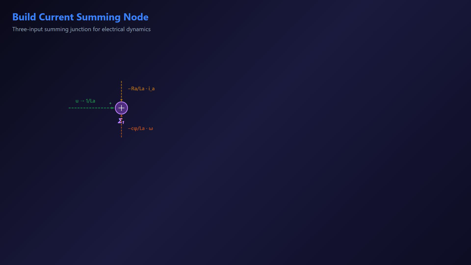
The early diagram frames are partial construction stages; faded paths await their source signals. The speed-sum step uses the clean speed-equation card as an algebraic reference. The final diagram contains two integrators and three negative contributions. Compact integrals suppress their initial-value constants.
Build the current summing junction.
Combine the voltage, resistive and back-EMF contributions.
Current-node output:
$\displaystyle i_{a}'\left(t\right) = \left(\frac{1}{L_{a}}\right)\cdot u - \left(\frac{R_{a}}{L_{a}}\right)\cdot i_{a} - \left(\frac{c\cdot \varphi }{L_{a}}\right)\cdot \omega .$
Narration transcript
First, draw a summing junction for the current dynamics. It must combine three terms. Plus 1 over L A times U, minus R A over L A times I A, and minus C phi over L A times omega.
12. Scale the voltage input
The early diagram frames are partial construction stages; faded paths await their source signals. The speed-sum step uses the clean speed-equation card as an algebraic reference. The final diagram contains two integrators and three negative contributions. Compact integrals suppress their initial-value constants.
Create the positive voltage input path.
Route u through gain 1/L_a to the current junction.
Narration transcript
Create a forward input path. Root U through a gain block 1 over LA and connect it to the positive input of the current summing junction.
13. Return the resistive contribution
The early diagram frames are partial construction stages; faded paths await their source signals. The speed-sum step uses the clean speed-equation card as an algebraic reference. The final diagram contains two integrators and three negative contributions. Compact integrals suppress their initial-value constants.
Add the negative resistive contribution.
Return i_a through gain R_a/L_a to the negative current-junction input.
Narration transcript
Now add negative current feedback. Take IA from the current integrator output, pass it through gain RA over LA and feed it back to the same summing node with a minus sign.
14. Return the speed coupling
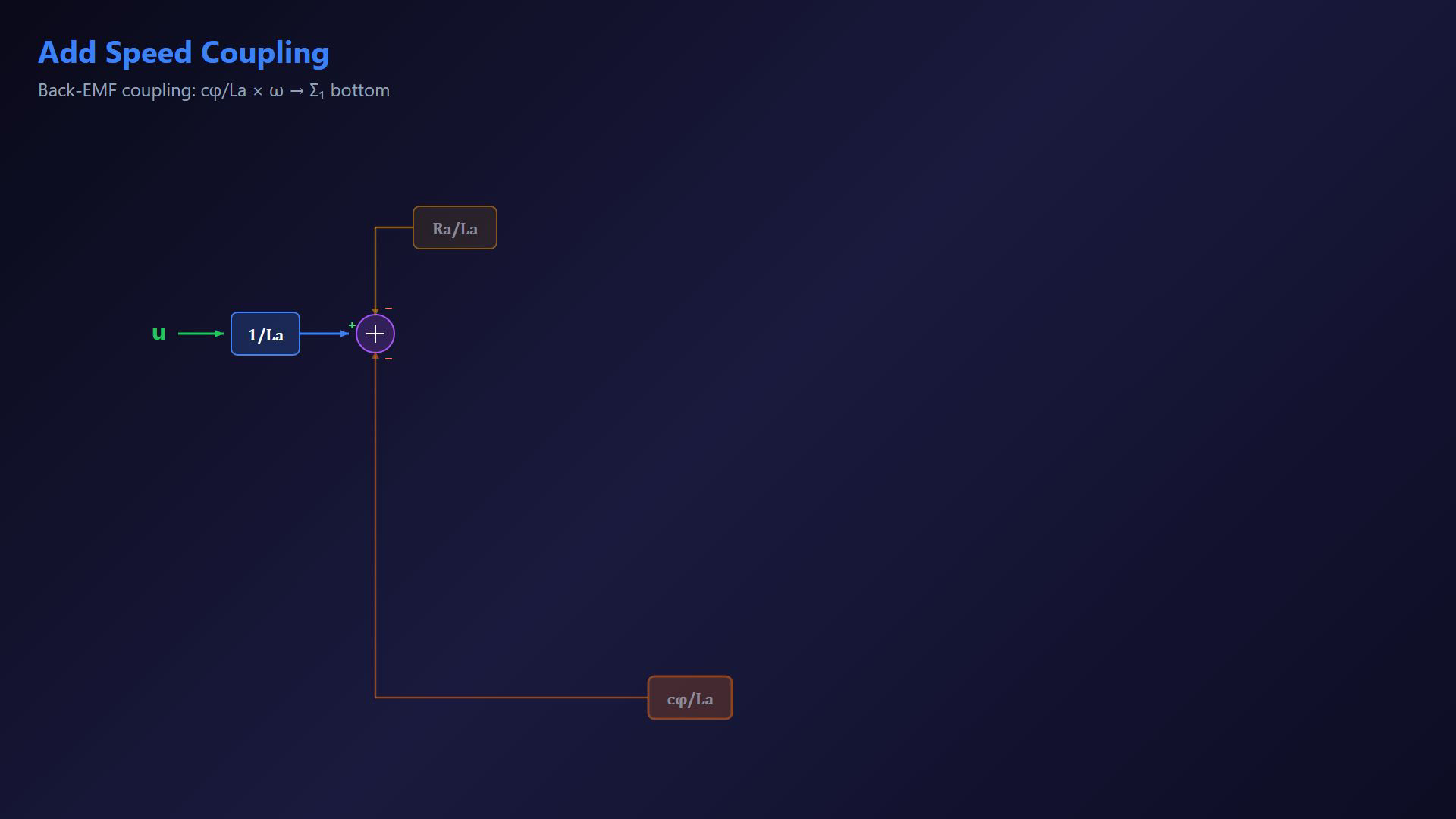
The early diagram frames are partial construction stages; faded paths await their source signals. The speed-sum step uses the clean speed-equation card as an algebraic reference. The final diagram contains two integrators and three negative contributions. Compact integrals suppress their initial-value constants.
Add the back-EMF coupling contribution.
Return ω through gain (c·φ)/L_a to the negative current-junction input.
Keep this coupling sign negative.
Narration transcript
Add the electromechanical coupling term. Take omega, pass it through gain C phi over LA and feed it negatively to the current summing node. Sign placement is critical here.
15. Integrate the current derivative
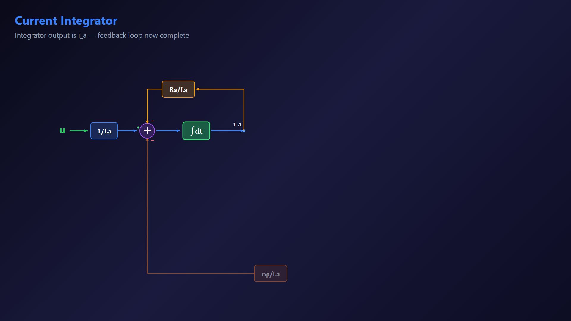
The early diagram frames are partial construction stages; faded paths await their source signals. The speed-sum step uses the clean speed-equation card as an algebraic reference. The final diagram contains two integrators and three negative contributions. Compact integrals suppress their initial-value constants.
Integrate the current-node output with the specified initial current.
The first integrator produces armature current i_a.
Branch i_a to the resistive path and the mechanical torque path.
Narration transcript
The output of the current summing node enters an integrator 1 over s. The integrator output is ia. This signal branches to other parts of the diagram.
16. Build the speed summing node
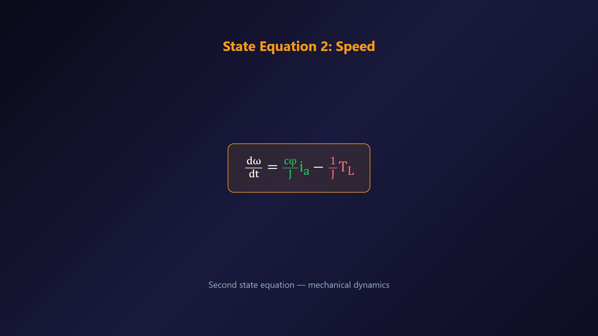
The early diagram frames are partial construction stages; faded paths await their source signals. The speed-sum step uses the clean speed-equation card as an algebraic reference. The final diagram contains two integrators and three negative contributions. Compact integrals suppress their initial-value constants.
Build the mechanical summing junction; use the equation card as a reference.
Combine motor torque and opposing load torque after scaling by inertia.
Speed-node output:
$\displaystyle \omega '\left(t\right) = \left(\frac{c\cdot \varphi }{J}\right)\cdot i_{a} - \left(\frac{1}{J}\right)\cdot T_{L}.$
Narration transcript
Next, draw the speed dynamic summing junction. It has two inputs. plus Cφ over J times Ia and minus 1 over J times TL.
17. Add motor torque contribution
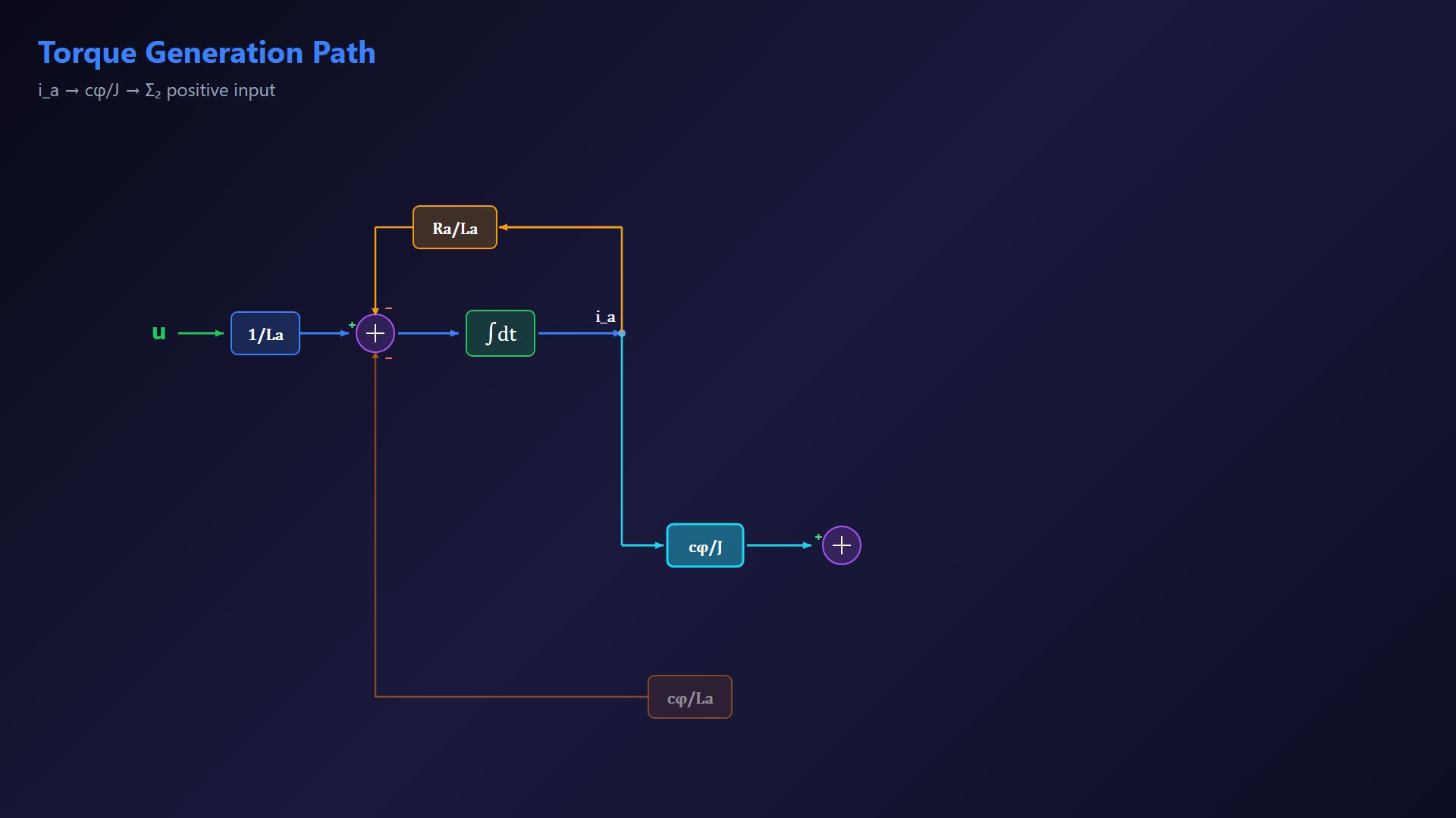
The early diagram frames are partial construction stages; faded paths await their source signals. The speed-sum step uses the clean speed-equation card as an algebraic reference. The final diagram contains two integrators and three negative contributions. Compact integrals suppress their initial-value constants.
Pass i_a through gain (c·φ)/J to the positive mechanical input.
This contribution accelerates the motor in the chosen positive direction.
Narration transcript
From Ia, add gain Cφ over J and connect it to the positive input of the speed summing node. This path represents motor torque contribution to acceleration.
18. Subtract load torque
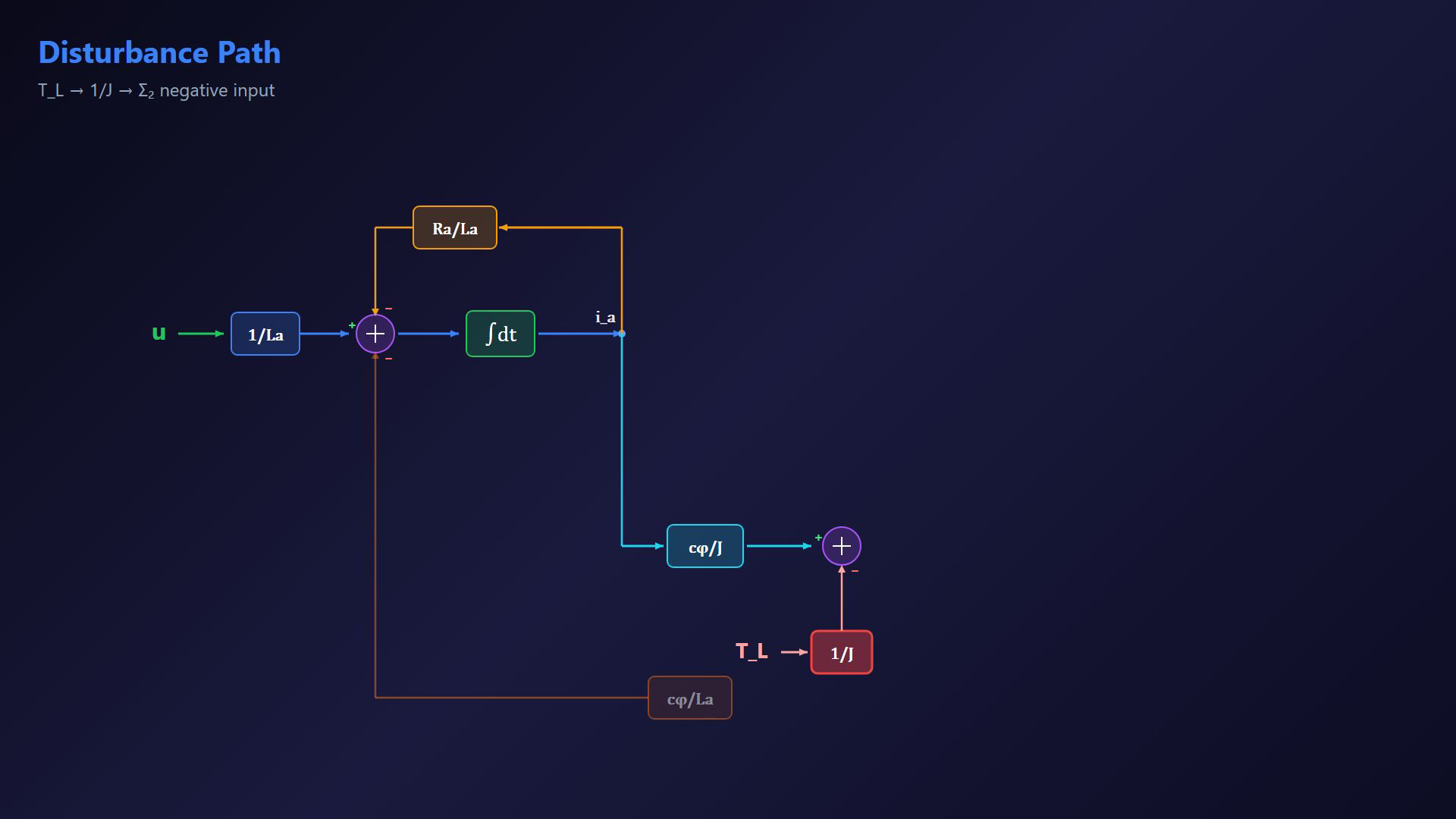
The early diagram frames are partial construction stages; faded paths await their source signals. The speed-sum step uses the clean speed-equation card as an algebraic reference. The final diagram contains two integrators and three negative contributions. Compact integrals suppress their initial-value constants.
Add the opposing load-torque disturbance.
Pass T_L through gain 1/J to the negative mechanical input.
Narration transcript
Now, add the disturbance path. Load torque TL enters through gain 1 over J and connects with a negative sign to the speed summing node.
19. Integrate the speed derivative
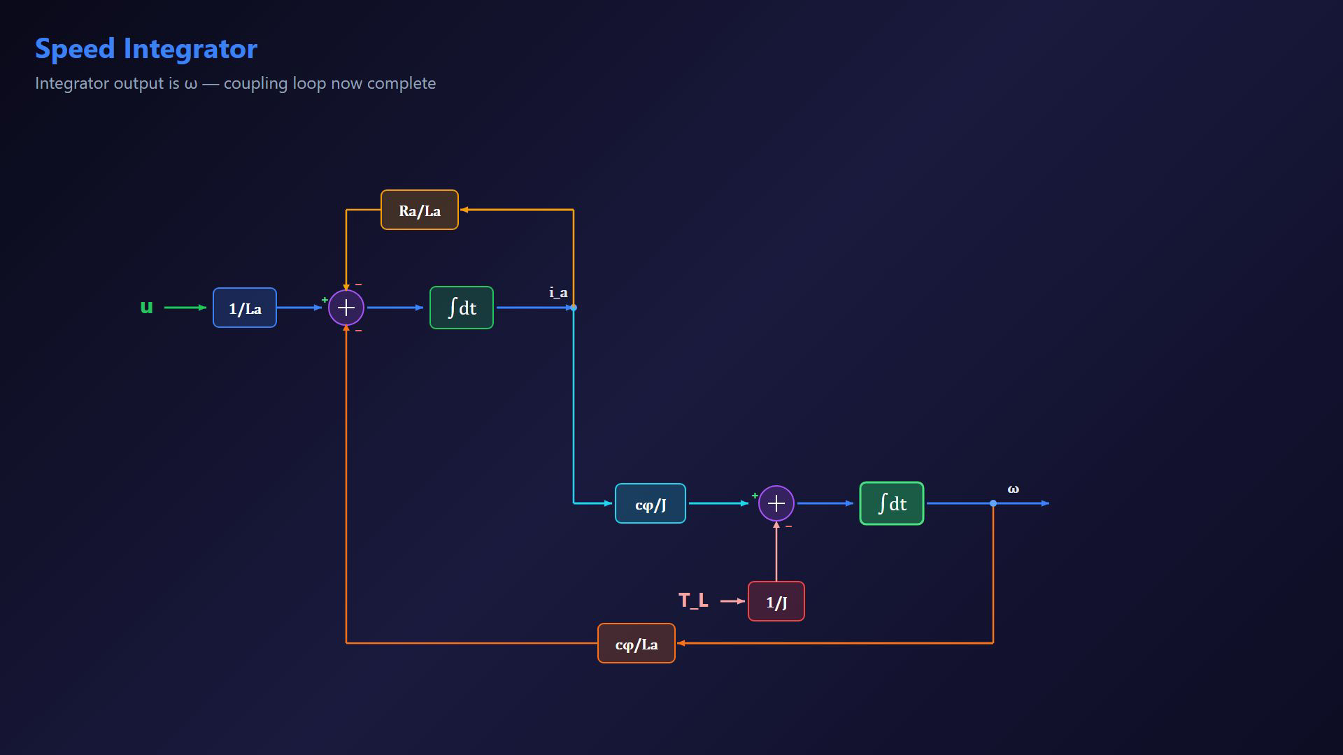
The early diagram frames are partial construction stages; faded paths await their source signals. The speed-sum step uses the clean speed-equation card as an algebraic reference. The final diagram contains two integrators and three negative contributions. Compact integrals suppress their initial-value constants.
Integrate the speed-node output with the specified initial speed.
The second integrator produces angular speed ω.
Narration transcript
The speed summing output goes through another integrator 1 over S. The integrator output is omega, which is also our output Y.
20. Identify output speed
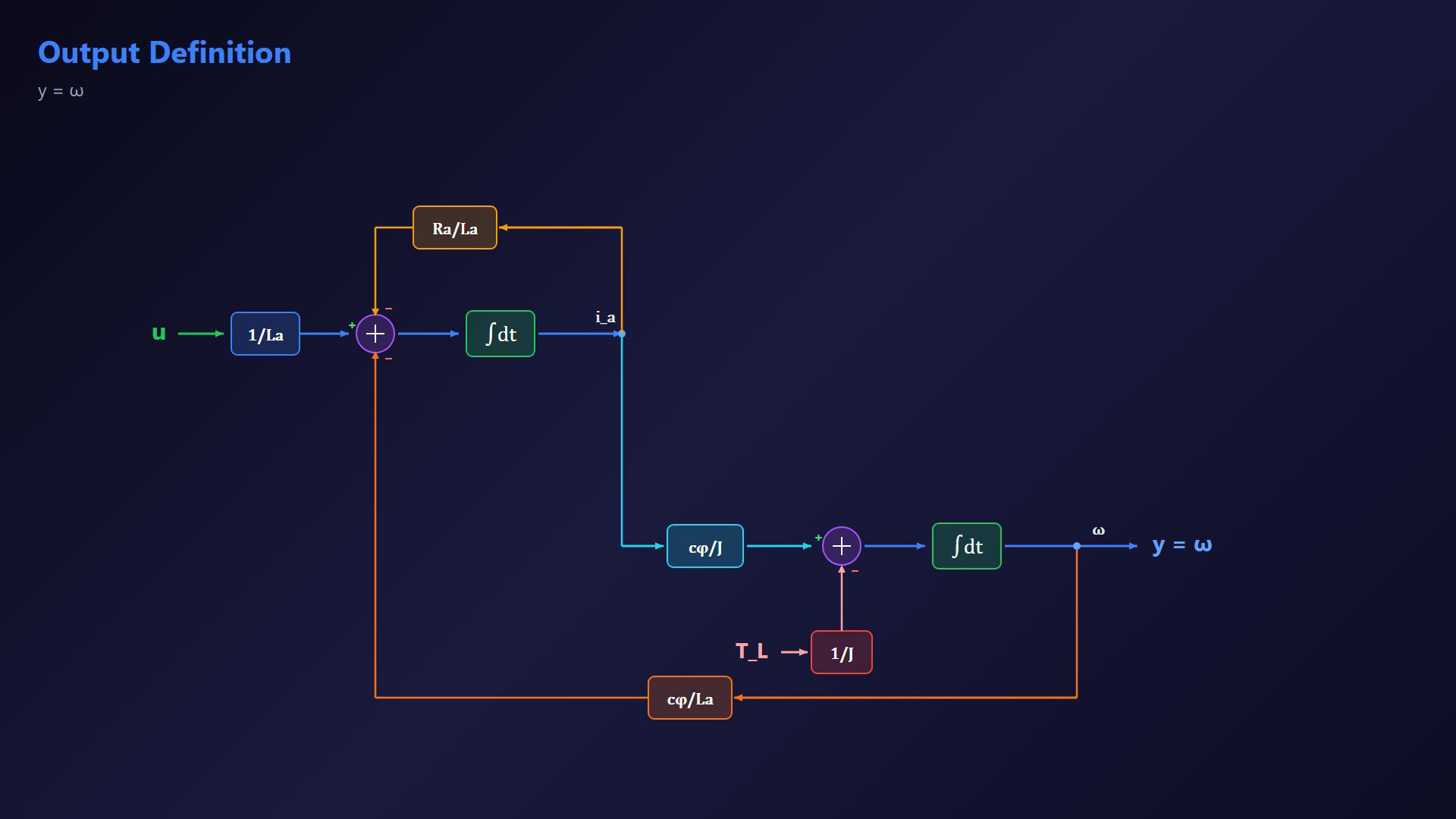
The early diagram frames are partial construction stages; faded paths await their source signals. The speed-sum step uses the clean speed-equation card as an algebraic reference. The final diagram contains two integrators and three negative contributions. Compact integrals suppress their initial-value constants.
Output definition:
$\displaystyle y = \omega .$
Use the same output notation consistently.
Narration transcript
Mark the output clearly as Y equals omega. This keeps notation consistent with previous lessons where Y was the measured output signal.
21. Check signs and directions
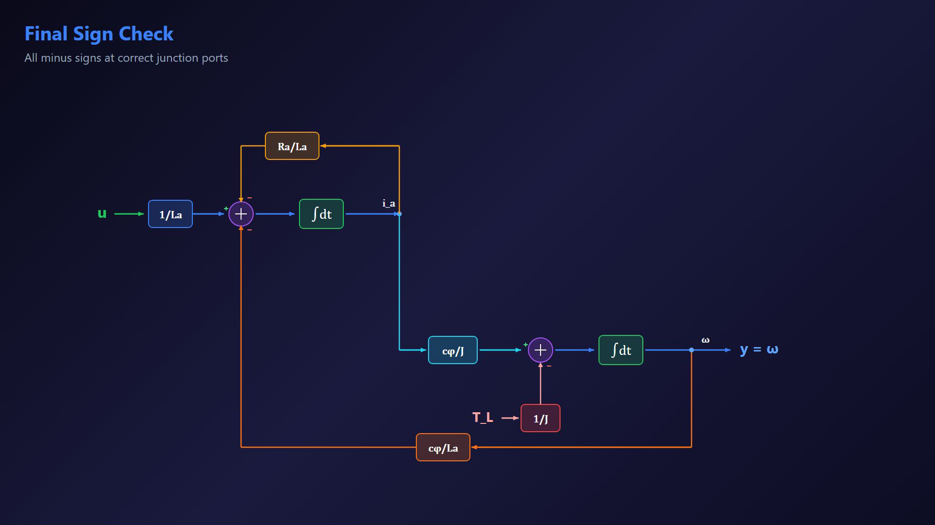
The early diagram frames are partial construction stages; faded paths await their source signals. The speed-sum step uses the clean speed-equation card as an algebraic reference. The final diagram contains two integrators and three negative contributions. Compact integrals suppress their initial-value constants.
Check every junction sign and signal arrow.
Subtract resistive drop and back EMF electrically; subtract load torque mechanically.
Narration transcript
Before finalizing, check every sign and arrow direction. Resistive and back EMF terms must subtract in the electrical loop and load torque must subtract in the mechanical loop.
22. Read the completed model
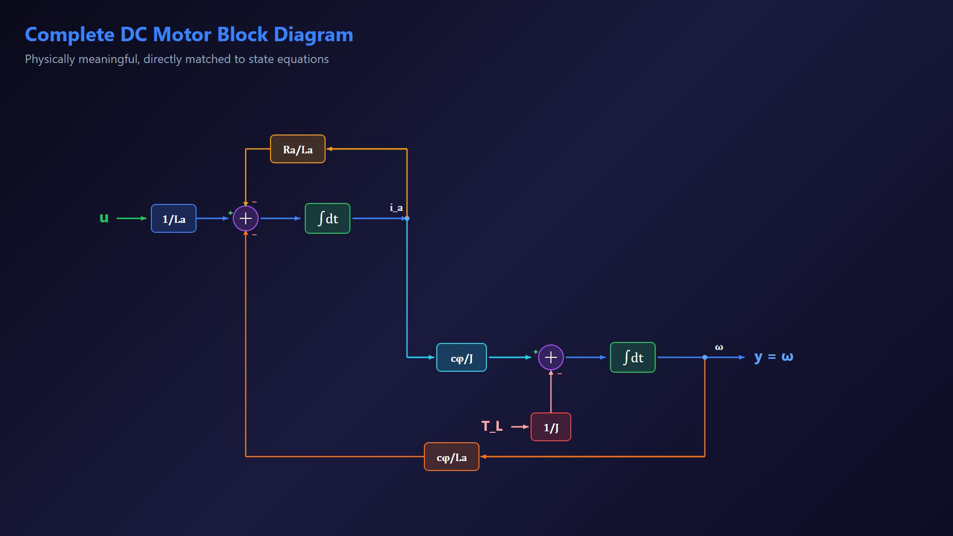
The early diagram frames are partial construction stages; faded paths await their source signals. The speed-sum step uses the clean speed-equation card as an algebraic reference. The final diagram contains two integrators and three negative contributions. Compact integrals suppress their initial-value constants.
Read the complete two-state motor diagram and its disturbance input.
Match every path to its state-equation term.
Narration transcript
Now we have the full DC motor block diagram with disturbance input. The structure is compact, physically meaningful and directly matched to the state equations.
23. Preserve equivalent operations
The early diagram frames are partial construction stages; faded paths await their source signals. The speed-sum step uses the clean speed-equation card as an algebraic reference. The final diagram contains two integrators and three negative contributions. Compact integrals suppress their initial-value constants.
Equivalent layouts preserve gains, signs, signal flow and matched initial states.
Narration transcript
In practice, equivalent diagrams may look different in layout, but they remain mathematically identical if gains, signs, and signal flow are preserved.
24. Review the two-state realization
The early diagram frames are partial construction stages; faded paths await their source signals. The speed-sum step uses the clean speed-equation card as an algebraic reference. The final diagram contains two integrators and three negative contributions. Compact integrals suppress their initial-value constants.
Review the construction.
Model both physical parts, derive two state equations and connect their integrator realization.
Continue to the next lesson.
Narration transcript
Great work. In this lesson, we modeled a coupled electrical mechanical system, derived state equations, and converted them into a correct block diagram. See you in the next lesson.