Control Theory · Check the Pole Condition Before Computing a Step-Response Final Value

#36 Compare two quadratic denominators differing only by the constant-term sign

Use the final-value theorem for the stable system and prove divergence from the uncanceled positive pole of the second system.

Question

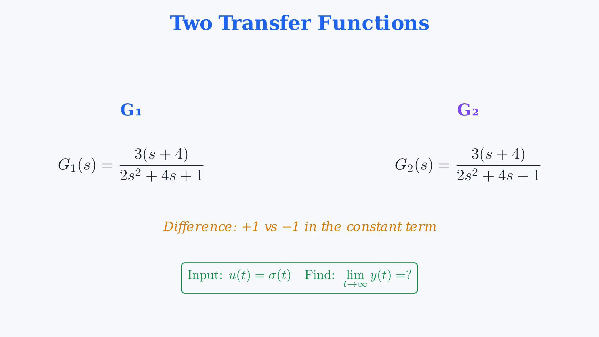
Whole existing final-video frame showing the two transfer functions, the final-value pole condition, the stable quadratic roots or the valid steady-state calculation. — The numerator is three times the entire bracket s plus four. Check the reduced poles of sY before interpreting an algebraic value at zero as a finite long-time output.

Find the zero-state output limit for a positive unit step applied to each continuous-time real rational transfer function G1(s)=3(s+4)/(2s²+4s+1) and G2(s)=3(s+4)/(2s²+4s-1). The numerator is three times the entire bracket s+4, not 3s+4. This grouping is explicit in the problem and substitution figures and in the spoken follow-up three times four equals twelve. The sole difference between the denominators is+1 versus-1. The symbol sigma(t) in the problem figure denotes the unit step: zero for t<0 and one for t>0; its isolated value at zero does not affect these ordinary Laplace calculations. No physical units, nonzero initial conditions, hidden state realization or feedback interconnection is specified. For this zero-state unit-step experiment U(s)=1/s, Y(s)=G(s)/s and sY(s)=G(s). For these strictly proper reduced rational responses, a finite final value is obtained from the limit of sY(s) as s approaches zero from the right only after verifying that every pole of reduced sY(s) lies strictly in the open left half plane. Then the time-domain limit as t grows without bound equals G(0). A simple pole of Y at the origin, coming from a constant final output, is removed by the factor s; that is why the criterion concerns sY, not Y alone. Repeated origin or remaining imaginary-axis poles would need attention, and a genuine right-half-plane pole with nonzero residue produces growth. Here the numerators do not cancel any denominator root: their only zero is-4, where the denominators equal17 and15. Both are strictly proper, so no impulsive output from a polynomial part needs interpretation. This input-output statement does not establish stability of hidden nonminimal states. The source's derivative explanation is intuition within the present rational response class, not a theorem for arbitrary smooth convergent functions. Convergence of y(t) alone does not imply that yprime(t) tends to zero; for example sin(t²)/t tends to zero while its derivative oscillates for t>=1. For the actual stable rational response, the remaining modes are decaying exponentials, whose derivatives also decay. The unilateral derivative identity uses the initial value consistent with the one-sided convention; here y(0-)=y(0+)=0. Likewise s approaching zero is not a pointwise substitution for time going to infinity. The limit relation requires the pole condition. When the source says the theorem gives a wrong number, read this as an invalid use of an algebraic substitution outside the theorem's hypotheses; the valid theorem has not failed. For G1, the denominator is2s²+4s+1. A real quadratic a2*s²+a1*s+a0 with all three coefficients nonzero and of the same sign has both roots strictly in the left half plane. Dividing out a common negative sign is harmless. Its ordinary Routh first column is(a2,a1,a0); no zero pivot or row arises here. The column(2,4,1) has no sign changes. This same-sign shortcut is for a quadratic; positivity of all coefficients alone does not ensure stability at arbitrary higher orders. The quadratic formula gives(-4 plus or minus sqrt(16-8))/4=(-4 plus or minus sqrt8)/4=-1 plus or minus sqrt2/2. The two poles are approximately-0.292893 and-1.707107; the source rounds them to-0.29 and-1.71. Thus FVT applies to this unit-step response. Substitute zero with all grouping intact: numerator3(0+4)=12 and denominator2*0²+4*0+1=1. The finite final output is12. The initial animation illustrates a different generic underdamped system settling near one; it is not a plot of either stated transfer function. Stability in general does not require an increasing or monotonic step response. More specifically, the source's possible-overshoot wording in the G1 section is too broad for these fixed coefficients. This particular G1 rises monotonically to12 and does not overshoot. To verify, let r=sqrt2/2, p=-1+r and q=-1-r. Its impulse response, which is the derivative of the unit-step response for t>0, is C*exp(p*t)+D*exp(q*t), with C=3/4+9/(4r)>0 and D=3/4-9/(4r)<0. Since p>q and C+D=3/2>0, this derivative remains positive: factor exp(q*t) and note C*exp((p-q)*t)+D>=C+D. The output starts at zero and has limit12, so it stays below12. Damping and the zero determine the shape jointly, and neither is a free parameter after this transfer function is fixed. The notebook explicitly qualifies this source wording without changing either given function or its final-value answer. For G2, the denominator is2s²+4s-1. With positive leading coefficient its root product is-1/2, so the roots are real and have opposite signs. The discriminant16+8=24 is strictly positive. The roots are(-4 plus or minus sqrt24)/4=-1 plus or minus sqrt6/2, approximately+0.224745 and-2.224745. The first positive pole is not canceled by the zero at-4. Its Routh first column(2,4,-1) also has one sign change. Hence reduced sY has a right-half-plane pole and the finite final-value theorem does not apply. Algebraic substitution gives G2(0)=12/(-1)=-12; this identity is arithmetically correct but does not equal the output's long-time limit. To establish the actual behavior rather than infer it from an invalid limit substitution, let p=-1+sqrt6/2>0 and q=-1-sqrt6/2<0. Partial fractions give Y2(s)=-12/s+A/(s-p)+B/(s-q), where A=3(p+4)/[2p(p-q)]>0 and B=3(q+4)/[2q(q-p)]. Thus y2(t)=-12+A*exp(p*t)+B*exp(q*t) for t>=0. The constant coefficient is the same-12 found algebraically, but the positive-pole contribution grows and is nonzero; it cannot be dropped. In fact this particular positive unit-step response tends to positive infinity, so it has no finite real limit. The source's0.22 and2.22 values are rounded pole approximations, not exact exponents to use in a precise asymptotic equivalence. Use the exact radicals for that purpose. A stable but undamped-pole exception or other input is a separate problem; do not generalize the summary's grows-unbounded phrase to every system outside strict BIBO stability. Keep the final rule precise: identify the actual reduced sY, check its poles, then compute a finite final value only when the hypotheses hold.

Written solution and narration transcript(shows the full solution)

Below are all the lines written in the notebook together with the full narration transcript.

1. Separate the illustrative step response from the given systems
The numerator is three times the entire bracket s plus four. Check the reduced poles of sY before interpreting an algebraic value at zero as a finite long-time output.
The opening curve illustrates a stable step response; stability alone does not require a rising or monotone output.
We seek the finite output limit as time grows without bound.
Use a transfer-function limit after verifying the final-value theorem conditions.
Narration transcript
When we apply a step input to a stable system, the output rises and eventually settles at a final value. That final value, y of infinity, is what we want to find. Today we will use the final value theorem to compute it directly from the transfer function, without solving any differential equations.
2. Read the two transfer functions and unit-step input
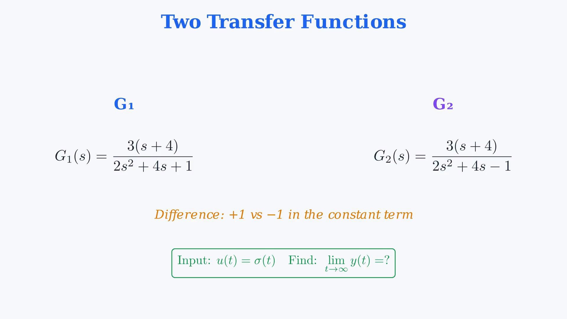
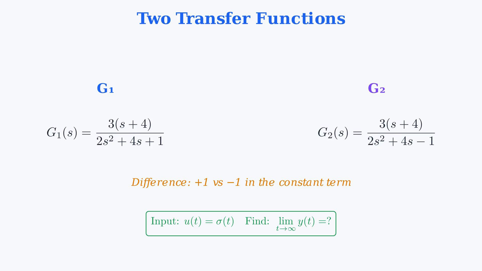
The numerator is three times the entire bracket s plus four. Check the reduced poles of sY before interpreting an algebraic value at zero as a finite long-time output.
Read the problem.
Compare the two stated zero-state transfer functions.
First function with grouped numerator:
$\displaystyle G_{1}\left(s\right) = 3\cdot \frac{s+4}{2\cdot s^{2}+4\cdot s+1}$
Second function with grouped numerator:
$\displaystyle G_{2}\left(s\right) = 3\cdot \frac{s+4}{2\cdot s^{2}+4\cdot s-1}$
Only the constant-term sign differs between the denominators.
Apply a unit step to each system from rest.
Find whether the long-time output has a finite limit and, if so, its value.
Narration transcript
Here is our problem. We are given two transfer functions. G1 of s equals 3 times s plus 4, divided by 2 s squared plus 4 s plus 1. G2 of s equals 3 times s plus 4, divided by 2 s squared plus 4 s minus 1. Notice that the only difference is the sign of the last term in the denominator, plus 1 versus minus 1. For both systems, a unit step input is applied. We need to find the limit of y of t as t goes to infinity.
3. State the final-value theorem and its pole condition
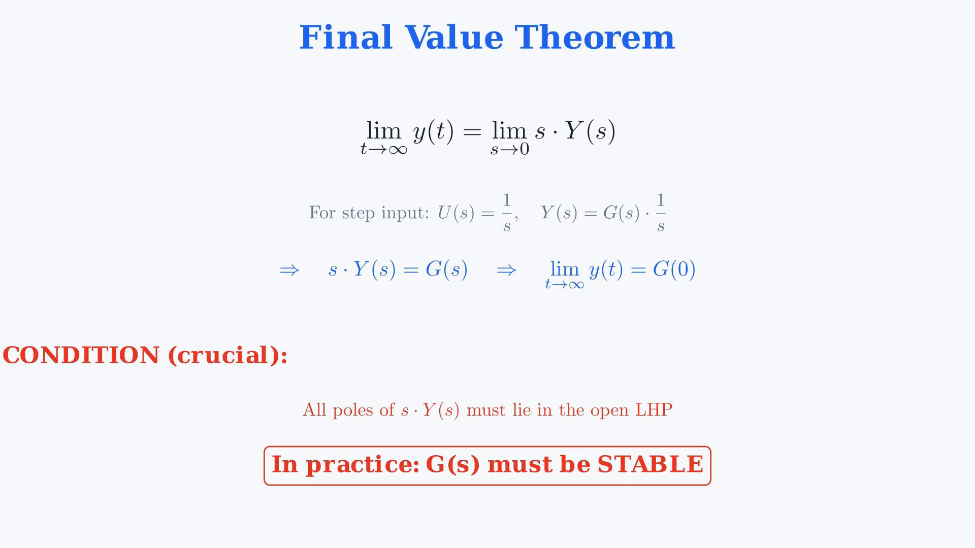
The numerator is three times the entire bracket s plus four. Check the reduced poles of sY before interpreting an algebraic value at zero as a finite long-time output.
Under its pole condition, the time-domain final limit equals the limit of s times the output transform as s approaches zero from the right.
Understand the limit relation together with its assumptions.
Unilateral derivative identity for the present zero initial output:
$\displaystyle L\{y'\left(t\right)\} = s\cdot Y\left(s\right)-y\left(0\right)$
For this stable rational response, the decaying modes and their derivatives tend to zero; convergence alone would not prove this for an arbitrary function.
Small transform parameter and large time are connected by a conditional limit theorem, not a pointwise substitution.
Keep this derivative argument as intuition after the pole check.
Unit-step transforms:
$\displaystyle U\left(s\right) =\frac{ 1}{s}; Y\left(s\right) =\frac{ G\left(s\right)}{s}$
Cancel the step factor:
$\displaystyle s\cdot Y\left(s\right) = G\left(s\right)$
When the pole condition holds:
$\displaystyle y\left(\infty \right) = G\left(0\right)$
Check the critical hypothesis.
Every pole of reduced s times the output transform must lie strictly in the open left half plane for this rational-response criterion.
Here the condition reduces to stability of the proper reduced transfer function.
An uncanceled positive-real-part pole in the actual output transform contributes a nonzero growing mode.
Outside the hypotheses, a substituted number is not a theorem result.
Check the reduced poles first, then evaluate at zero if the condition holds.
Always perform the stability check.
Narration transcript
The final value theorem states that the limit of y of t as t goes to infinity equals the limit of s times Y of s as s goes to zero. Why does this work? Recall that the Laplace transform of a derivative is s times Y of s minus the initial value y of zero. If y of t approaches a steady value, its derivative approaches zero. Taking s to zero in the Laplace domain corresponds to taking t to infinity in the time domain. That is the intuition behind the theorem. For a unit step input, U of s equals 1 over s, and Y of s equals G of s times 1 over s. So s times Y of s simplifies to G of s. Therefore y of infinity equals G of zero. But there is a critical condition. All poles of s times Y of s must lie in the open left half plane, otherwise the limit does not exist. In practice, this means the transfer function G of s must be stable. If the system has a pole with positive real part, the output contains a growing exponential term and does not approach a finite value. The final value theorem gives a number, but that number is wrong. So the plan is: first check stability, then if stable, compute G of zero. Never skip the stability check.
4. Verify both poles of the stable quadratic
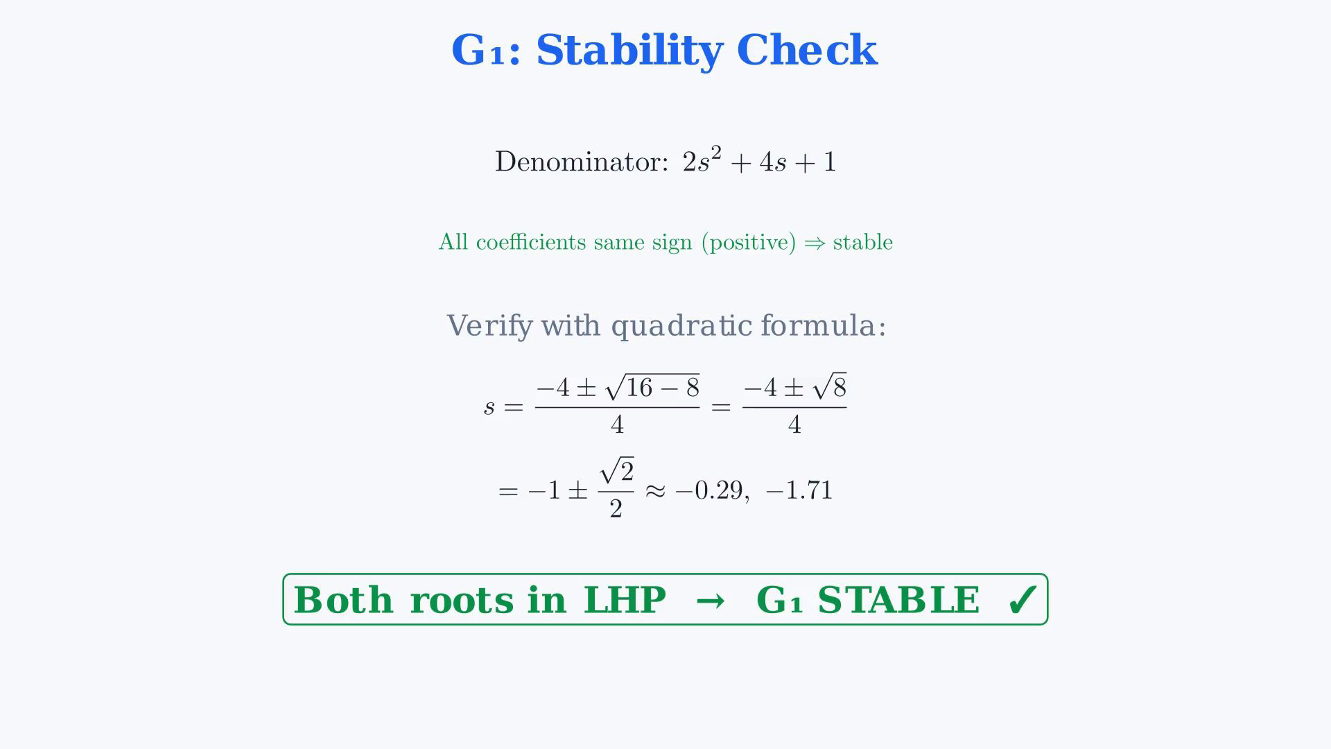
The numerator is three times the entire bracket s plus four. Check the reduced poles of sY before interpreting an algebraic value at zero as a finite long-time output.
Check the first system.
First denominator:
$\displaystyle D_{1}\left(s\right) = 2\cdot s^{2}+4\cdot s+1$
For a real quadratic, three nonzero coefficients of the same sign imply strict left-half-plane roots.
All three coefficients here are positive.
This quadratic shortcut follows from the Routh-Hurwitz criterion.
Routh first column:
$\displaystyle v_{1} = \left(2,4,1\right)$
Verify the roots independently.
Quadratic formula:
$\displaystyle s =\frac{-4\pm \sqrt{16-8}}{4}$
Simplify the discriminant:
$\displaystyle s =\frac{-4\pm \sqrt{8}}{4}$
Exact poles:
$\displaystyle s = -1\pm \frac{\sqrt{2}}{2}$
The two poles round to minus zero point two nine and minus one point seven one.
Both poles have strictly negative real parts.
The first transfer function is strictly proper and stable, with no cancellations to inspect further.
The final-value theorem applies to its unit-step response.
Narration transcript
Check stability of G1. The denominator is 2 s squared plus 4 s plus 1. For a second order polynomial, there is a quick rule: if all three coefficients have the same sign, the system is stable. Here all three are positive, so G1 is stable by inspection. This shortcut comes from the Routh-Hurwitz criterion applied to a second order polynomial. The first column of the Routh array is just the three coefficients themselves, so no sign change means no right half plane pole. Let us verify with the quadratic formula for certainty. The roots are s equals negative 4 plus or minus the square root of 16 minus 8, all divided by 4. That is negative 4 plus or minus the square root of 8, divided by 4. Simplifying, s equals negative 1 plus or minus the square root of 2 divided by 2. Numerically, the roots are approximately negative 0.29 and negative 1.71. Both have negative real parts, so both are in the left half plane. Stability is confirmed. FVT can be safely applied.
5. Evaluate the valid limit and interpret the actual response
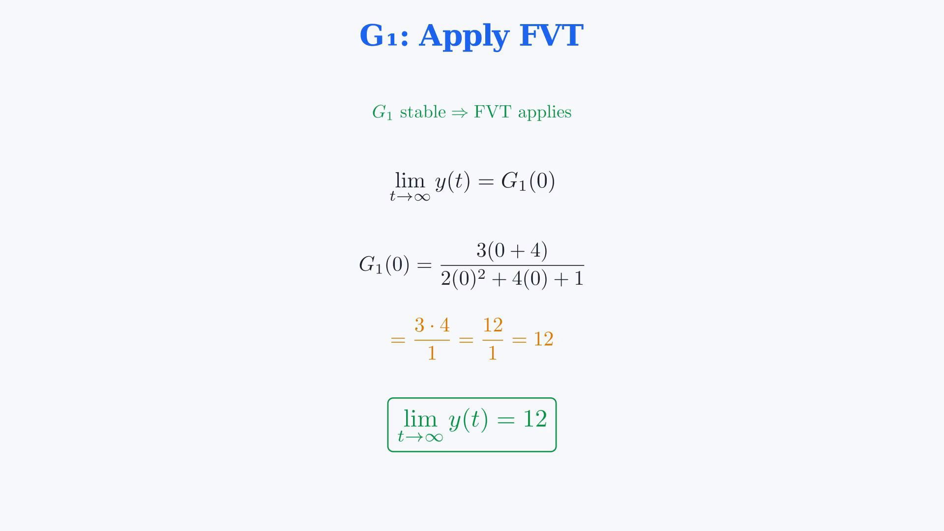
The numerator is three times the entire bracket s plus four. Check the reduced poles of sY before interpreting an algebraic value at zero as a finite long-time output.
Apply the theorem to the first system.
Its verified pole condition permits the limit calculation.
Valid finite final value:
$\displaystyle y\left(\infty \right) = G_{1}\left(0\right)$
Substitute the transform variable:
$\displaystyle s = 0$
Keep the full numerator bracket:
$\displaystyle N_{1}\left(0\right) = 3\cdot \left(0+4\right) = 12$
Evaluate the denominator:
$\displaystyle D_{1}\left(0\right) = 2\cdot 0^{2}+4\cdot 0+1 = 1$
Compute the ratio:
$\displaystyle y\left(\infty \right) =\frac{ 12}{1 }= 12$
The finite final output is twelve.
For these exact coefficients the response rises monotonically to twelve; the source's possible-overshoot wording is too broad for this particular function.
The given coefficients and zero already fix the shape; the verified steady value remains twelve.
Narration transcript
Now apply the final value theorem to G1. Since G1 is stable, the theorem holds. y of infinity equals G1 of zero. Plug in s equals zero. The numerator becomes 3 times zero plus 4, which is 3 times 4, which is 12. The denominator becomes 2 times zero squared plus 4 times zero plus 1, which reduces to just 1. So y of infinity equals 12 divided by 1, which equals 12. That is our answer for G1. The step response of G1 starts at zero, rises, possibly overshoots, and eventually settles to the horizontal line at y equals 12 as time grows large. The exact shape depends on damping, but the steady state value is unambiguous: 12.
6. Find the positive pole of the second quadratic
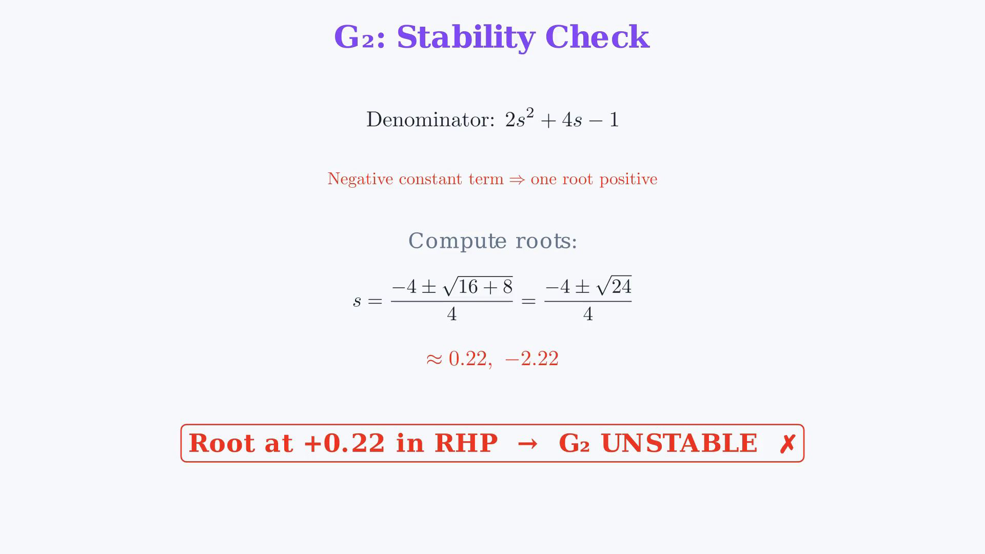
The numerator is three times the entire bracket s plus four. Check the reduced poles of sY before interpreting an algebraic value at zero as a finite long-time output.
Check the second system.
Second denominator:
$\displaystyle D_{2}\left(s\right) = 2\cdot s^{2}+4\cdot s-1$
The constant coefficient is now negative.
With positive leading coefficient, inspect the root product.
For this quadratic the root product is the constant coefficient divided by the leading coefficient.
Root product:
$\displaystyle p\cdot q = -\frac{1}{2}$
The negative product forces two real roots with opposite signs.
The positive root is an uncanceled right-half-plane pole.
Compute both roots explicitly.
Quadratic formula:
$\displaystyle s =\frac{-4\pm \sqrt{16+8}}{4}$
Simplify the discriminant:
$\displaystyle s =\frac{-4\pm \sqrt{24}}{4}$
The poles round to positive zero point two two and negative two point two two.
The positive pole makes this transfer function unstable.
The finite final-value theorem does not apply.
Narration transcript
Check stability of G2. The denominator is 2 s squared plus 4 s minus 1. Notice that the constant term is now negative. This is an immediate red flag. For a second order polynomial with leading coefficient positive, the product of the roots equals the constant term divided by the leading coefficient. Here the product is negative one half, a negative number. Negative product means one root positive, one root negative. And a positive root is a pole in the right half plane, which makes the system unstable. Let us compute the roots explicitly. Using the quadratic formula, s equals negative 4 plus or minus the square root of 16 plus 8, all divided by 4. That is negative 4 plus or minus the square root of 24, divided by 4. Numerically, s is approximately 0.22 and negative 2.22. The root at positive 0.22 is in the right half plane, so G2 is unstable. The final value theorem does not apply.
7. Show why the growing mode prevents a finite limit
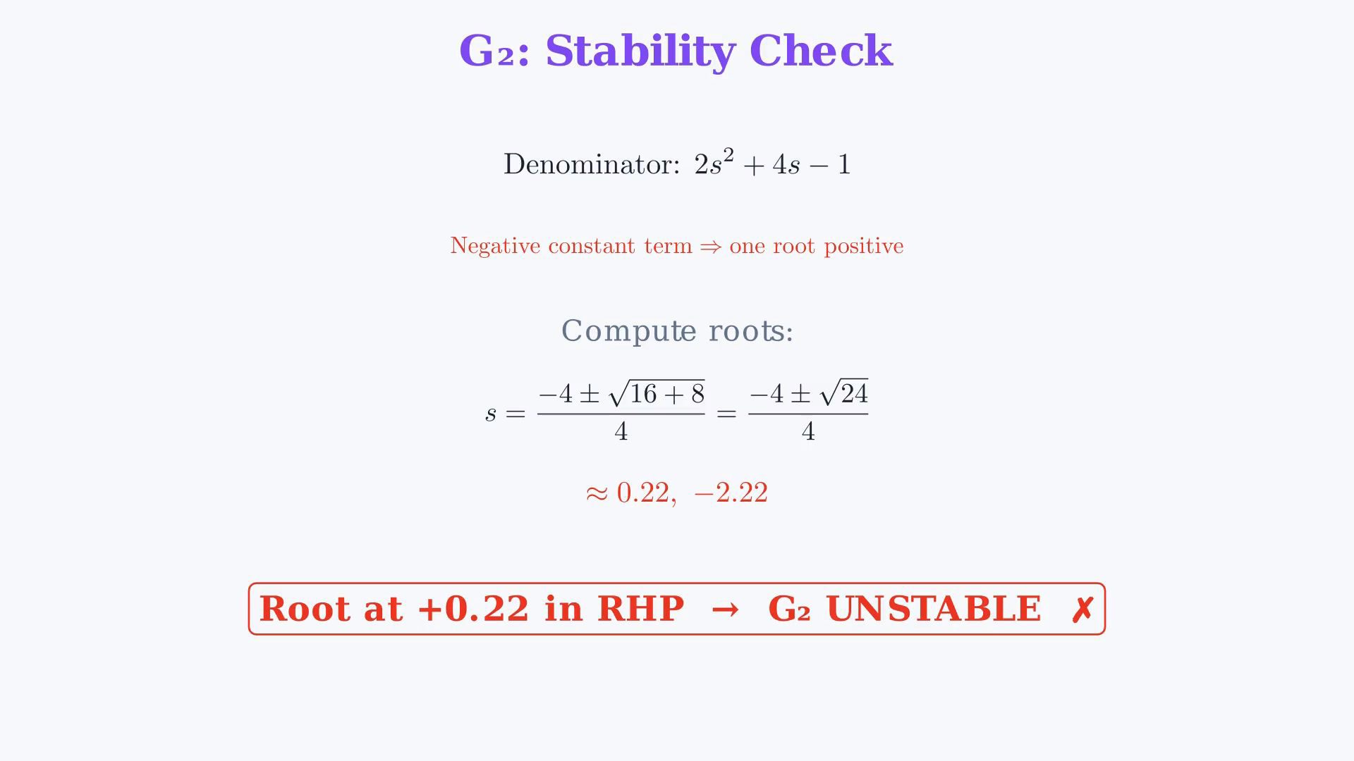
The numerator is three times the entire bracket s plus four. Check the reduced poles of sY before interpreting an algebraic value at zero as a finite long-time output.
The second function fails the pole condition.
Algebraic identity only, not a final output:
$\displaystyle G_{2}\left(0\right) =\frac{ 12}{-1}= -12$
The value minus twelve is not the long-time output limit.
Examine the actual partial fractions to identify the growing mode.
Use the exact two poles in the output transform:
$\displaystyle Y_{2}\left(s\right) = -\frac{12}{s}+\frac{A}{s-p}+\frac{B}{s-q}$
Each simple pole contributes its corresponding exponential or constant term.
The origin-pole contribution is the constant:
$\displaystyle y_{0}\left(t\right) = -12$
The negative pole gives a decaying contribution:
$\displaystyle y_{\mathrm{decay}}\left(t\right) = B\cdot e^{q\cdot t}$
The positive pole gives a growing contribution:
$\displaystyle y_{\mathrm{grow}}\left(t\right) = A\cdot e^{p\cdot t}$
Its coefficient is nonzero and positive, so this growing exponential dominates.
This particular positive unit-step output grows without bound toward positive infinity.
There is no finite real output limit.
Verify the pole condition before using the final-value theorem.
An algebraic value at zero cannot replace the absent finite limit.
Narration transcript
Since G2 is unstable, the final value theorem does not apply. You might be tempted to just plug in s equals zero anyway: G2 of zero equals 12 divided by negative 1, equals negative 12. But this number is completely meaningless for our problem. Let us see why by thinking about what y of t actually looks like. When we take the inverse Laplace transform of Y of s, which is G2 of s times 1 over s, we do partial fraction expansion and end up with terms like one over s, one over s minus 0.22, and one over s plus 2.22. Each term in the s-domain corresponds to a time function. The one over s term gives a constant. The one over s plus 2.22 term gives a decaying exponential. But the one over s minus 0.22 term gives e to the positive 0.22 t, which grows without bound as t increases. This growing exponential dominates the response. The output diverges. The limit of y of t as t goes to infinity does not exist. Lesson learned: always verify stability before applying the final value theorem. Without stability, the theorem gives you a finite number that has absolutely nothing to do with the true long-term behavior.
8. Compare a valid final value with divergence
The numerator is three times the entire bracket s plus four. Check the reduced poles of sY before interpreting an algebraic value at zero as a finite long-time output.
Compare the two results.
For these zero-state unit-step experiments, use the value at zero only after the proper reduced transfer function passes the pole condition.
The first quadratic has strictly negative poles.
First system final value:
$\displaystyle y_{1}\left(\infty \right) = G_{1}\left(0\right) = 12$
The second quadratic has one uncanceled positive pole.
The second response tends to positive infinity and has no finite final value.
Check the actual reduced poles first, then apply the theorem within its hypotheses.
Narration transcript
Let us summarize. The final value theorem gives y of infinity equal to G of zero for a step input, but only when G of s is stable. For G1, all denominator coefficients are positive, so G1 is stable. y of infinity equals G1 of zero equals 12. For G2, the constant term is negative, so one root is in the right half plane, G2 is unstable. The output diverges, the limit does not exist. Always check stability first, then apply the theorem.