Control Theory · Impulse Response and Convolution

#11 Connect zero-state continuous-time LTI impulse responses, convolution and Laplace products

Derive an admissible input response by convolution or Laplace multiplication, then check a causal first-order lag and an integrator.

Question

Existing lesson frame illustrating an impulse response, convolution integral or Laplace transform pair. — Use the continuous-time LTI zero-state setting. The Dirac arrow represents unit area, not an ordinary infinite-valued function. Causal examples use the unit step H(t). The first-order example uses the clean Laplace-pair card as an algebraic reference; it does not show a first-order response curve.

Work with a continuous-time linear time-invariant system and its zero-state input-output channel. The impulse response characterizes that channel, not arbitrary nonzero initial states, hidden internal modes, nonlinear systems or time-varying systems. The Dirac impulse is a distribution: its action on a smooth test function is the value of that function at zero. Unit-area narrow pulses illustrate its limit. Infinite amplitude and zero width are informal shorthand; do not evaluate zero times infinity or treat the impulse as an ordinary function with a numeric height. The arrow label denotes unit area. For the causal unilateral Laplace convention integrate from zero minus so an impulse at the origin is included fully; do not assign it an arbitrary half weight. The impulse response g and transfer function G form a transform pair on the stated domain. A bilateral rational expression alone does not specify a unique time signal without a region of convergence or causality: 1/s with real part of s positive represents H(t), whereas the left-sided branch with real part of s negative represents minus H of minus t. H denotes the unit step, distinct from the general input u. In the causal zero-state examples use the right-sided branch. The convolution integral runs over the whole real line when it exists, or is defined in an appropriate distribution framework. Arbitrary input means an admissible input for which the operation exists, not an arbitrary divergent expression. As a function of the integration variable tau, g of t minus tau is reflected and then shifted, not merely translated. If both input and impulse response are causal, the ordinary integral reduces to zero through t for nonnegative t and vanishes for negative t. Treat any impulses at integration boundaries with the stated distribution convention. Laplace convolution becomes multiplication only where the transforms and convolution theorem apply. The Laplace variable s is complex frequency sigma plus j omega; a Fourier response on the imaginary axis additionally requires the appropriate convergence or distribution conditions. Multiplication by the transfer function describes the zero-state contribution; add the zero-input response when initial energy is nonzero. Inverse transformation must respect the chosen causality and region of convergence. For the first-order lag take a positive time constant T and constant gain K: G(s) is K divided by the whole denominator one plus s times T. The causal impulse response is K/T times exp of minus t/T times H(t), with region of convergence real part of s greater than minus 1/T for nonzero K. For a unit-step input H(t), U(s) is 1/s and the zero-state step response is K times one minus exp of minus t/T, multiplied by H(t). Its initial value is zero, its right initial slope is K/T, and for positive K it is concave downward, approaching K. The algebraic reference card is not a plot of this curve. A nonzero initial output adds its initial value times exp of minus t/T to the first-order response for nonnegative t. For the causal integrator G(s) is 1/s on real part of s positive and g(t) is H(t), equal to one for positive t and zero for negative t. The source phrase constant describes this positive-time branch; a constant on the entire real line convolved with a finite-area input gives that full area independent of t, not a running integral. The actual integrator card has bounds zero to t, supporting the causal interpretation. For causal ordinary inputs the zero-state output is the integral from zero to t of u(tau). A nonzero initial integrator value adds a constant. A unit-step input gives a ramp, so the ideal integrator is not BIBO stable. Neither existence of a transfer function nor characterization of a selected channel proves internal stability. Keep original narration distinct from these explicit mathematical qualifications.

Written solution and narration transcript(shows the full solution)

Below are all the lines written in the notebook together with the full narration transcript.

1. Introduce impulse response and convolution
Use the continuous-time LTI zero-state setting. The Dirac arrow represents unit area, not an ordinary infinite-valued function. Causal examples use the unit step H(t). The first-order example uses the clean Laplace-pair card as an algebraic reference; it does not show a first-order response curve.
Introduce impulse response and convolution.
Continue with Control Theory, Lesson 11.
Recall the zero-state transfer function G(s).
Connect a unit impulse to a general admissible-input response.
Narration transcript
Hello everyone. Welcome to lesson eleven. In the previous lesson we defined the transfer function G of s. Today we explore what happens when we apply a special input, the Dirac impulse, and how the system response leads to a general output formula through convolution.
2. Interpret the unit Dirac distribution
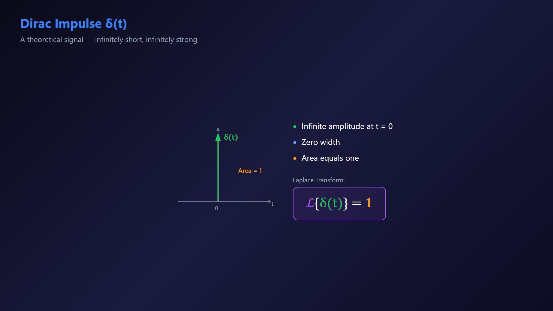
Use the continuous-time LTI zero-state setting. The Dirac arrow represents unit area, not an ordinary infinite-valued function. Causal examples use the unit step H(t). The first-order example uses the clean Laplace-pair card as an algebraic reference; it does not show a first-order response curve.
Interpret the Dirac impulse as a distribution.
Its unit area is a distribution property, not a product of zero width and infinite height.
Use a narrow unit-area pulse as an impulse-limit illustration.
Laplace transform of the full unit impulse:
$\displaystyle L\{\delta \left(t\right)\} = 1$
Narration transcript
The Dirac impulse delta of t is a theoretical signal. It has infinite amplitude at time zero, zero width, but its area equals one. Think of it as an infinitely short, infinitely strong kick applied to the system. Its Laplace transform is simply one.
3. Define the zero-state impulse response
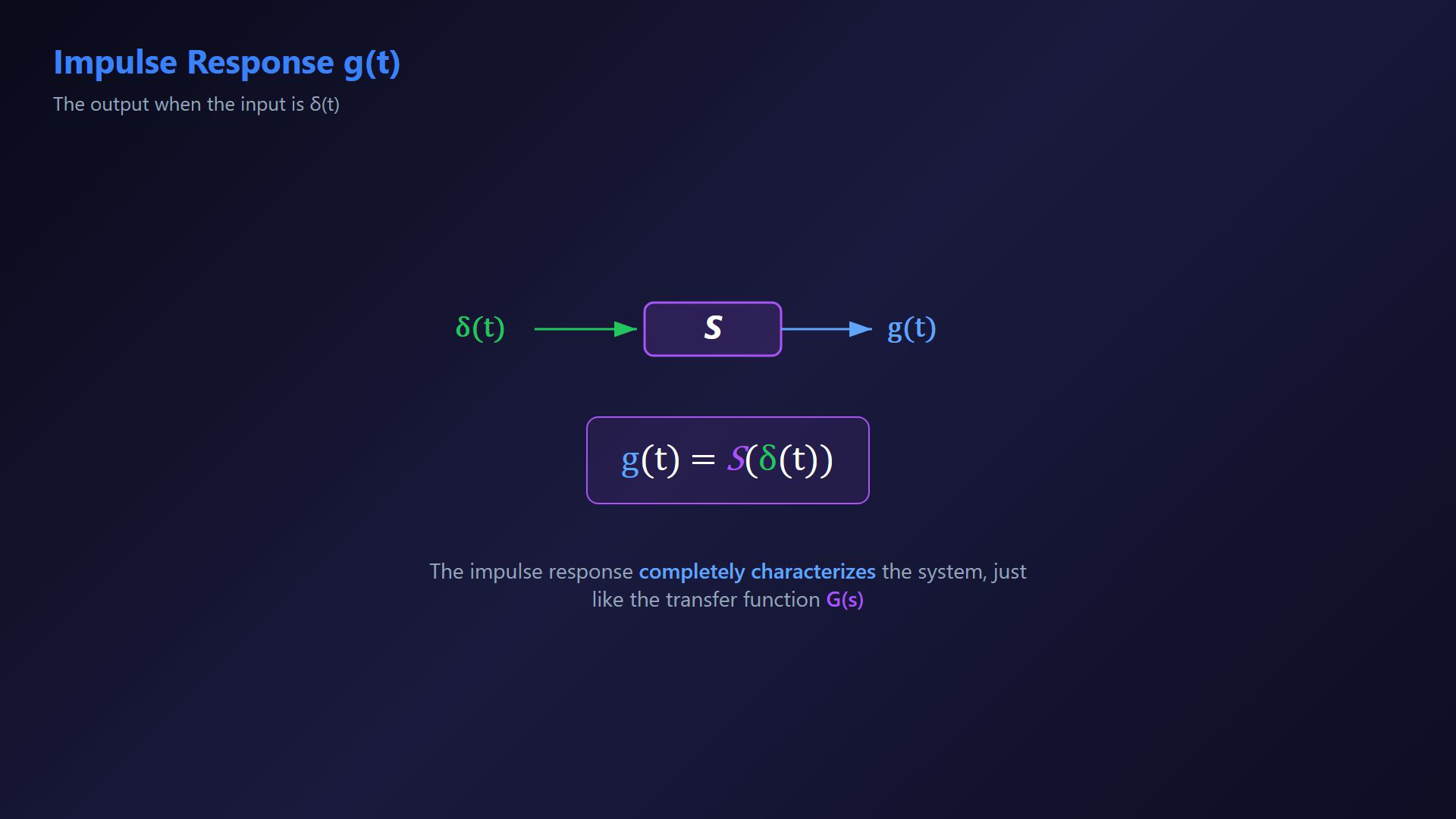
Use the continuous-time LTI zero-state setting. The Dirac arrow represents unit area, not an ordinary infinite-valued function. Causal examples use the unit step H(t). The first-order example uses the clean Laplace-pair card as an algebraic reference; it does not show a first-order response curve.
Apply a Dirac impulse to the continuous-time LTI system from zero state.
Impulse response:
$\displaystyle g\left(t\right) = S\{\delta \left(t\right)\}$
The impulse response characterizes this zero-state input-output channel.
Narration transcript
When we apply the Dirac impulse as input, the output is called the impulse response. We write g of t equals S of delta of t. The impulse response completely characterizes the system behavior, just like the transfer function does.
4. Relate g(t) to G(s)
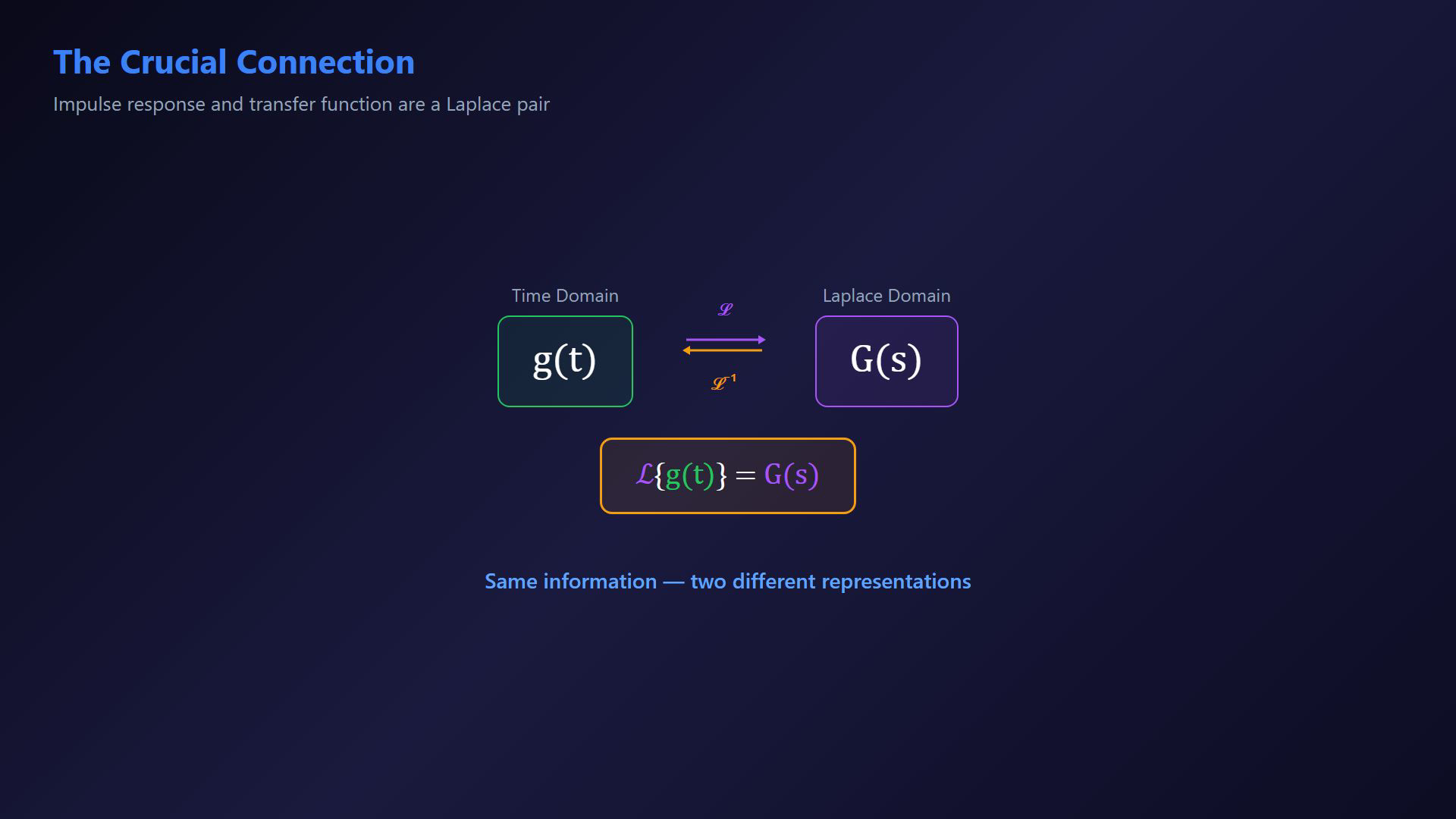
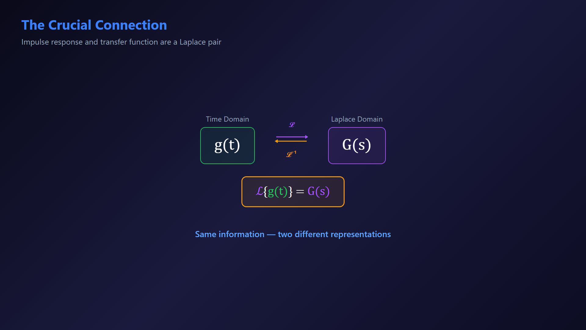
Use the continuous-time LTI zero-state setting. The Dirac arrow represents unit area, not an ordinary infinite-valued function. Causal examples use the unit step H(t). The first-order example uses the clean Laplace-pair card as an algebraic reference; it does not show a first-order response curve.
Connect the time and Laplace descriptions.
Use g(t) and G(s) as a Laplace pair on the specified convergence domain.
Transform pair:
$\displaystyle L\{g\left(t\right)\} = G\left(s\right)$
Include the causality or region-of-convergence information.
Narration transcript
Here is the crucial connection. The impulse response g of t and the transfer function G of s are a Laplace transform pair. Taking the Laplace transform of g of t gives G of s. This means the impulse response in time domain and the transfer function in Laplace domain contain exactly the same information.
5. Compute a response for an admissible input
Use the continuous-time LTI zero-state setting. The Dirac arrow represents unit area, not an ordinary infinite-valued function. Causal examples use the unit step H(t). The first-order example uses the clean Laplace-pair card as an algebraic reference; it does not show a first-order response curve.
Compute a practical output response.
Given g(t), find the zero-state output for an admissible input u(t).
Use convolution.
Narration transcript
Now we answer a practical question. If we know the impulse response g of t, how do we compute the output for any arbitrary input u of t? The answer is convolution.
6. Write the convolution integral
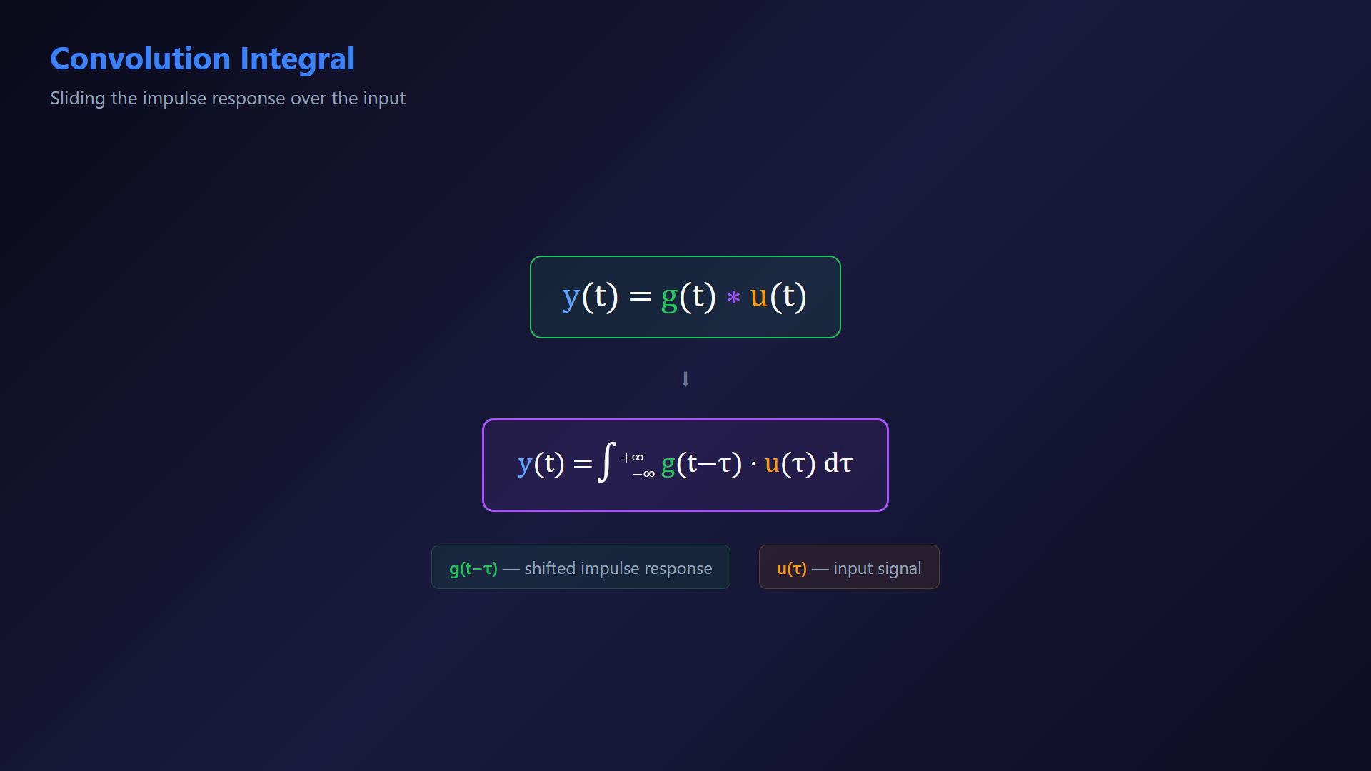
Use the continuous-time LTI zero-state setting. The Dirac arrow represents unit area, not an ordinary infinite-valued function. Causal examples use the unit step H(t). The first-order example uses the clean Laplace-pair card as an algebraic reference; it does not show a first-order response curve.
Zero-state convolution:
$\displaystyle y\left(t\right) = g\left(t\right) ∗ u\left(t\right)$
Full convolution integral:
$\displaystyle y\left(t\right) = \int _{-\infty }^{\infty } g\left(t-\tau \right)\cdot u\left(\tau \right) \mathrm{d}\tau$
Reflect and shift g as a function of τ, then integrate the weighted input contributions.
Narration transcript
The output y of t equals the convolution of g and u. Written as an integral, y of t equals the integral from minus infinity to plus infinity of g of t minus tau times u of tau, d tau. This integral slides the impulse response over the input and sums the weighted contributions.
7. Multiply the Laplace transforms
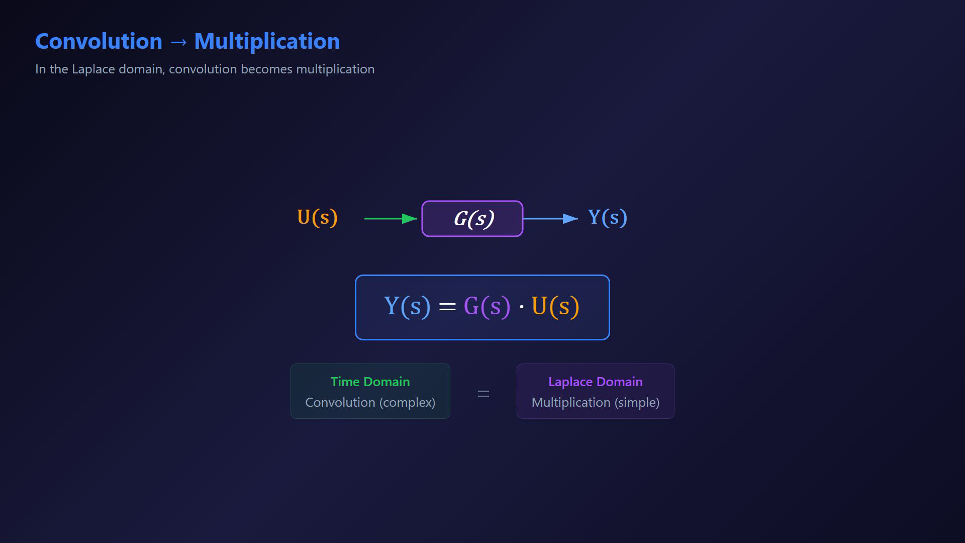
Use the continuous-time LTI zero-state setting. The Dirac arrow represents unit area, not an ordinary infinite-valued function. Causal examples use the unit step H(t). The first-order example uses the clean Laplace-pair card as an algebraic reference; it does not show a first-order response curve.
Apply the Laplace convolution theorem where the transforms exist.
Laplace product:
$\displaystyle Y\left(s\right) = G\left(s\right)\cdot U\left(s\right)$
Recover the same zero-state transfer relation.
Here the transform domain is the complex Laplace s domain.
Narration transcript
In the Laplace domain, convolution becomes simple multiplication. Y of s equals G of s times U of s. This is exactly the transfer function relationship we learned in the previous lesson. Convolution in time equals multiplication in frequency.
8. Recover the time-domain output
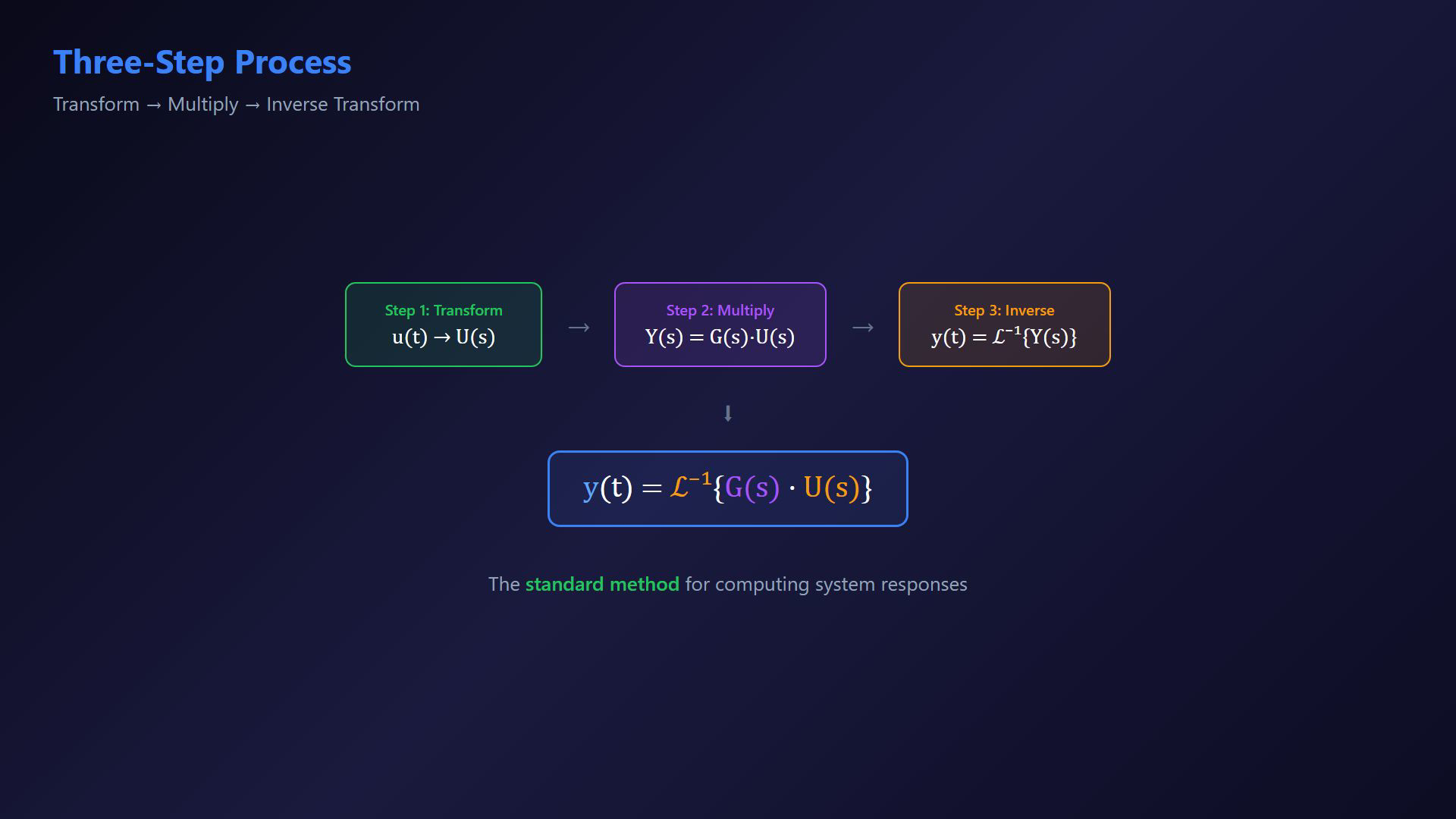
Use the continuous-time LTI zero-state setting. The Dirac arrow represents unit area, not an ordinary infinite-valued function. Causal examples use the unit step H(t). The first-order example uses the clean Laplace-pair card as an algebraic reference; it does not show a first-order response curve.
Recover the output by the inverse Laplace transform on the chosen causal branch.
Inverse transform:
$\displaystyle y\left(t\right) = L^{-1}\{Y\left(s\right)\} = L^{-1}\{G\left(s\right)\cdot U\left(s\right)\}$
Transform the input, multiply by G(s), then invert with the stated convergence conditions.
Narration transcript
To find the actual time domain output, we take the inverse Laplace transform. y of t equals the inverse Laplace of Y of s, which equals the inverse Laplace of G of s times U of s. This three step process, transform, multiply, inverse transform, is the standard method for computing system responses.
9. Check the first-order lag response
Use the continuous-time LTI zero-state setting. The Dirac arrow represents unit area, not an ordinary infinite-valued function. Causal examples use the unit step H(t). The first-order example uses the clean Laplace-pair card as an algebraic reference; it does not show a first-order response curve.
Check a causal first-order lag with positive time constant T and gain K.
Lag transform pair:
$\displaystyle G\left(s\right) =\frac{ K}{1+s\cdot T}, g\left(t\right) = \left(\frac{K}{T}\right)\cdot e^{-t/T}\cdot H\left(t\right)$
Zero-state unit-step response:
$\displaystyle y\left(t\right) = K\cdot \left(1-e^{-t/T}\right)\cdot H\left(t\right)$
Narration transcript
Let us see an example. For a first order lag with G of s equals K over one plus s T, the impulse response is g of t equals K over T times e to the minus t over T. Applying a step input and using the multiplication rule, we get the familiar step response K times one minus e to the minus t over T.
10. Check the causal integrator response
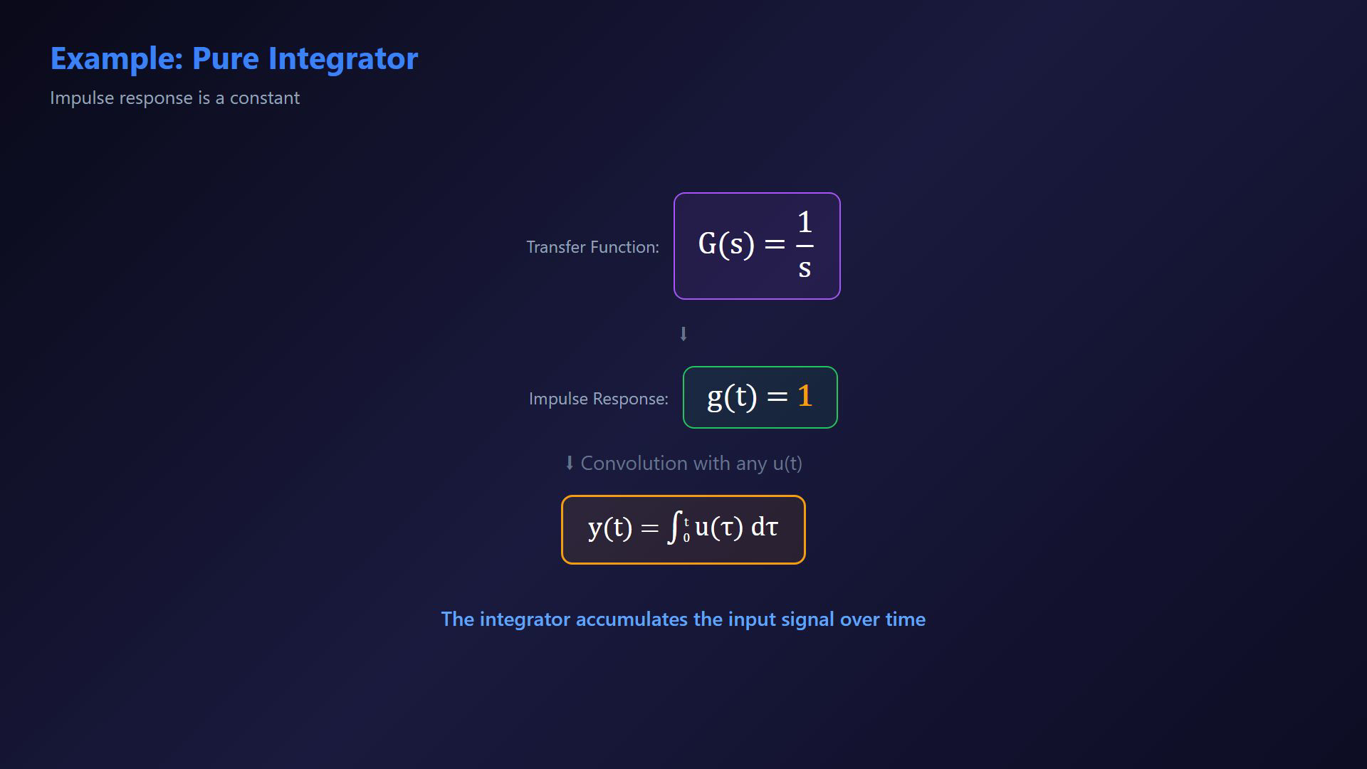
Use the continuous-time LTI zero-state setting. The Dirac arrow represents unit area, not an ordinary infinite-valued function. Causal examples use the unit step H(t). The first-order example uses the clean Laplace-pair card as an algebraic reference; it does not show a first-order response curve.
Causal integrator transfer:
$\displaystyle G\left(s\right) =\frac{ 1}{s}$
Causal impulse response:
$\displaystyle g\left(t\right) = H\left(t\right)$
For causal ordinary input and nonnegative t:
$\displaystyle y\left(t\right) = \int _{0}^{t} u\left(\tau \right) \mathrm{d}\tau$
The zero-state integrator accumulates the input; add the initial value if it is nonzero.
Narration transcript
For a pure integrator, G of s equals one over s. The impulse response is g of t equals one, a constant. Convolving a constant with any input gives the running integral of that input. This confirms that the integrator accumulates the input signal over time.
11. Review the LTI response model
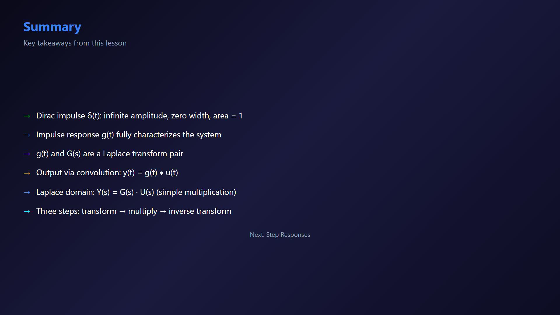
Use the continuous-time LTI zero-state setting. The Dirac arrow represents unit area, not an ordinary infinite-valued function. Causal examples use the unit step H(t). The first-order example uses the clean Laplace-pair card as an algebraic reference; it does not show a first-order response curve.
Review the result.
For the specified LTI zero-state channel, use the impulse-response pair and a well-defined convolution or Laplace product.
Continue with step responses.
Narration transcript
Great work. In this lesson we learned that the impulse response g of t fully characterizes a system, that g of t and G of s are Laplace pairs, and that the output for any input can be found by convolution in time or multiplication in the Laplace domain. See you in the next lesson on step responses.