Control Theory · Check an Equilibrium and Linearize the State and Output Maps
#32 Evaluate all three candidates, retain the output baseline and compute the four local coefficients
Build the local deviation model while distinguishing equilibrium, stability and the absolute output.
Question
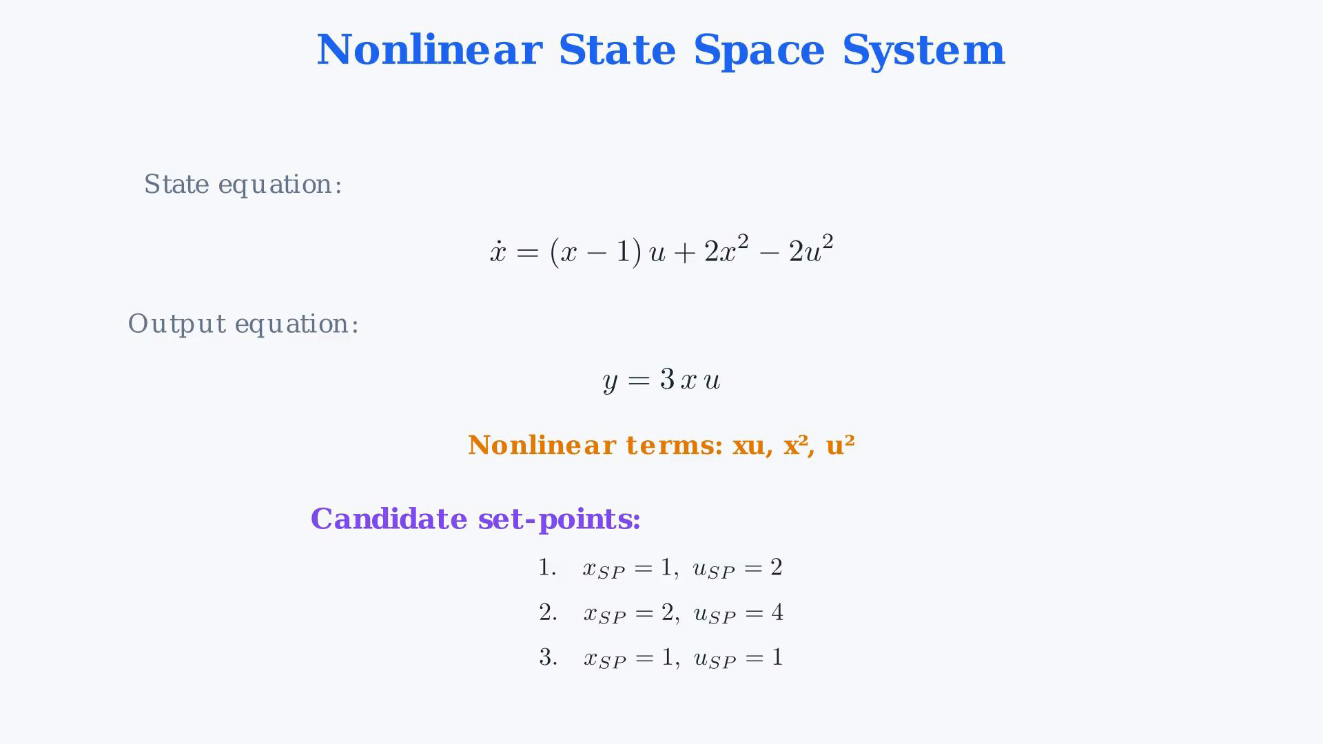
Consider the stated smooth continuous-time scalar nonlinear system x'=f(x,u)=(x-1)u+2x²-2u² and y=g(x,u)=3xu. The parentheses in (x-1)u are essential. The summary's shorter spoken wording is interpreted using the explicit quantity in the original problem and the correctly parenthesized original graphic. No numerical units or actuator limits are supplied; interpret the coefficients in the model's chosen coordinates and time units. This exercise asks for a constant equilibrium operating point and its local time-invariant deviation model. Hold each candidate input constant and require f(x_sp,u_sp)=0. Candidate1 is (1,2), giving0+2-8=-6. Candidate2 is (2,4), giving4+8-32=-20. Candidate3 is (1,1), giving0+2-2=0. Only the third of these three candidates satisfies the equilibrium condition. This does not mean it is the only equilibrium of the nonlinear system: (0,0), for example, is another equilibrium outside the supplied list. Also, equilibrium validity is not stability; an unstable equilibrium is still an equilibrium. The source's statement that a set-point must be an equilibrium is scoped to this constant equilibrium linearization. Smooth functions can also be Taylor expanded at a non-equilibrium point, but the resulting local model retains a nonzero constant drift f(x0,u0). Linearization about a moving nominal solution is another valid construction and generally gives time-varying coefficients. Neither of those is the equilibrium deviation model requested here. Do not reject all non-equilibrium Taylor expansions as impossible. At x_sp=1,u_sp=1, the absolute output baseline is y_sp=g(1,1)=3. Define the deviations Delta x=x-1, Delta u=u-1 and Delta y=y-3. The equilibrium values are constant, so the derivative of Delta x equals x'. In the notebook, xi,nu,eta may be used when explaining these same deviations; they do not denote extra states or inputs. The linearized equations describe the approximate first-order deviation model, not an exact replacement of the original nonlinear system for arbitrary excursions. Differentiate before evaluating. Holding u fixed, f_x=u+4x, which gives a=5 at(1,1). Holding x fixed, f_u=(x-1)-4u, which gives b=-4. For the output map, g_x=3u gives c=3 and g_u=3x gives d=3. The letters a,b,c,d here are scalar state-space coefficients, equivalently one-by-one matrices. Retain the negative sign in b and the nonzero direct output term d. The repeated spoken sentence 'At the set-point:3' is used once for each different output partial; both equal three. Thus the first-order model is (Delta x)'=5 Delta x-4 Delta u and Delta y=3 Delta x+3 Delta u. The latter is the deviation from3, so the approximate absolute output is y=3+3(x-1)+3(u-1). For a direct check, substitute x=1+xi and u=1+nu into the original polynomial. The exact state equation is xi'=5xi-4nu+xi nu+2xi²-2nu². The exact output deviation is eta=3xi+3nu+3xi nu. The omitted terms are quadratic in the small deviations. Scaling both deviations by a small factor scales the first-order terms by that factor and the omitted terms by its square; this describes local approximation accuracy, not a guarantee of accuracy for all later times. With the input held at its equilibrium value, the linearized state perturbation evolves as Delta x(t)=Delta x(0)e^(5t). The coefficient5 multiplies the state perturbation in the derivative equation; it does not instantaneously multiply the state itself by5. Because this smooth scalar equilibrium has a positive linearized eigenvalue, it is locally unstable with u held at1. Small perturbations can grow until the local approximation is no longer accurate. A negative b=-4 says a positive small input perturbation initially reduces the state derivative, with the state held fixed. Nonzero b gives control authority in this scalar local model; no feedback law or closed-loop stability is supplied by that fact. Likewise c=d=3 are equal numerical sensitivities in the stated coordinates, not an assertion that differently measured state and input increments have identical physical units. Keep the output's immediate direct input contribution separate from the subsequent state response.
Written solution and narration transcript(shows the full solution)
Below are all the lines written in the notebook together with the full narration transcript.
1. Read the nonlinear state and output maps
Keep the whole factor (x minus one) multiplied by u. The final model uses deviations from x=1, u=1 and y=3. Its positive state coefficient describes local open-loop instability. Read the nonlinear system.There is one state, one input and one output.State equation:Output equation:Both maps contain nonlinear terms.The state map contains a mixed product and two squared terms.The output contains a state-input product.Test the three candidates for a constant equilibrium deviation model.Narration transcript
Here is the problem. We have a nonlinear state space system. The state equation is x dot equals the quantity x minus 1 times u, plus 2 x squared, minus 2 u squared. The output equation is y equals 3 x u. Both equations are nonlinear. The state equation has mixed x u terms, x squared, and u squared. The output has an x u product. We are given three candidate set-points and need to determine which ones are suitable for linearization.
2. Check the three candidate equilibria
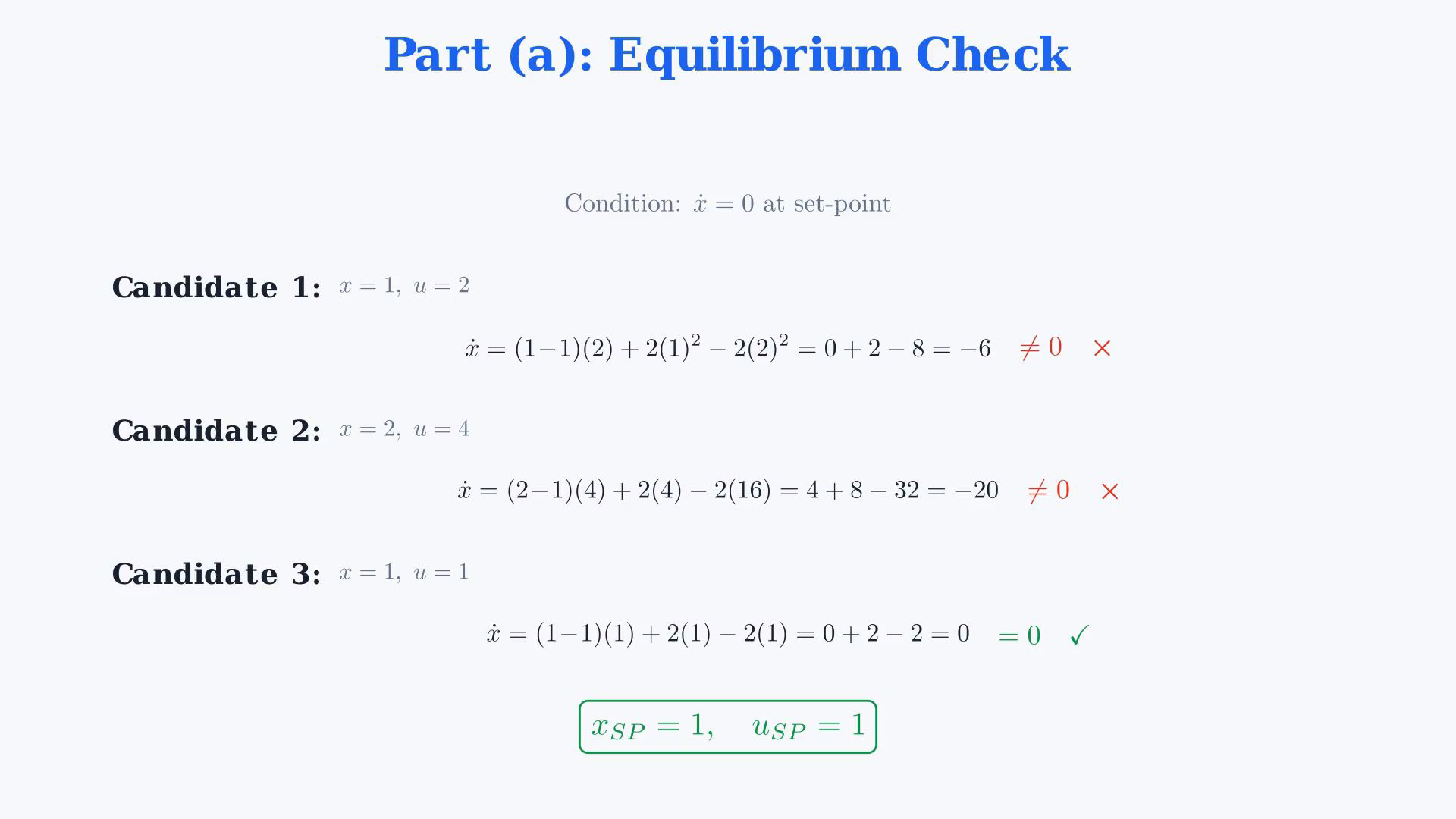
Keep the whole factor (x minus one) multiplied by u. The final model uses deviations from x=1, u=1 and y=3. Its positive state coefficient describes local open-loop instability. Equilibrium condition for the constant operating point:Substitute each complete candidate pair.Candidate one:Substitution:Residual:The first candidate is not an equilibrium.Candidate two:Substitution:Residual:The second candidate is not an equilibrium.Candidate three:Substitution:Residual:The third candidate satisfies the equilibrium test.Only candidate three among the supplied choices is valid; equilibrium does not imply stability.Narration transcript
For a set-point to be valid, the system must be in equilibrium, meaning x dot equals zero. Let us check each candidate. Candidate 1: x equals 1 and u equals 2. Substituting into x dot: the quantity 1 minus 1 times 2, plus 2 times 1 squared, minus 2 times 2 squared. That is 0 plus 2 minus 8, equals negative 6. Not zero, so candidate 1 is not valid. Candidate 2: x equals 2 and u equals 4. Substituting: the quantity 2 minus 1 times 4, plus 2 times 4, minus 2 times 16. That is 4 plus 8 minus 32, equals negative 20. Not zero, not valid. Candidate 3: x equals 1 and u equals 1. Substituting: the quantity 1 minus 1 times 1, plus 2 times 1, minus 2 times 1. That is 0 plus 2 minus 2, equals zero. Perfect. Candidate 3 is our valid set-point.
3. Compute all four partial derivatives
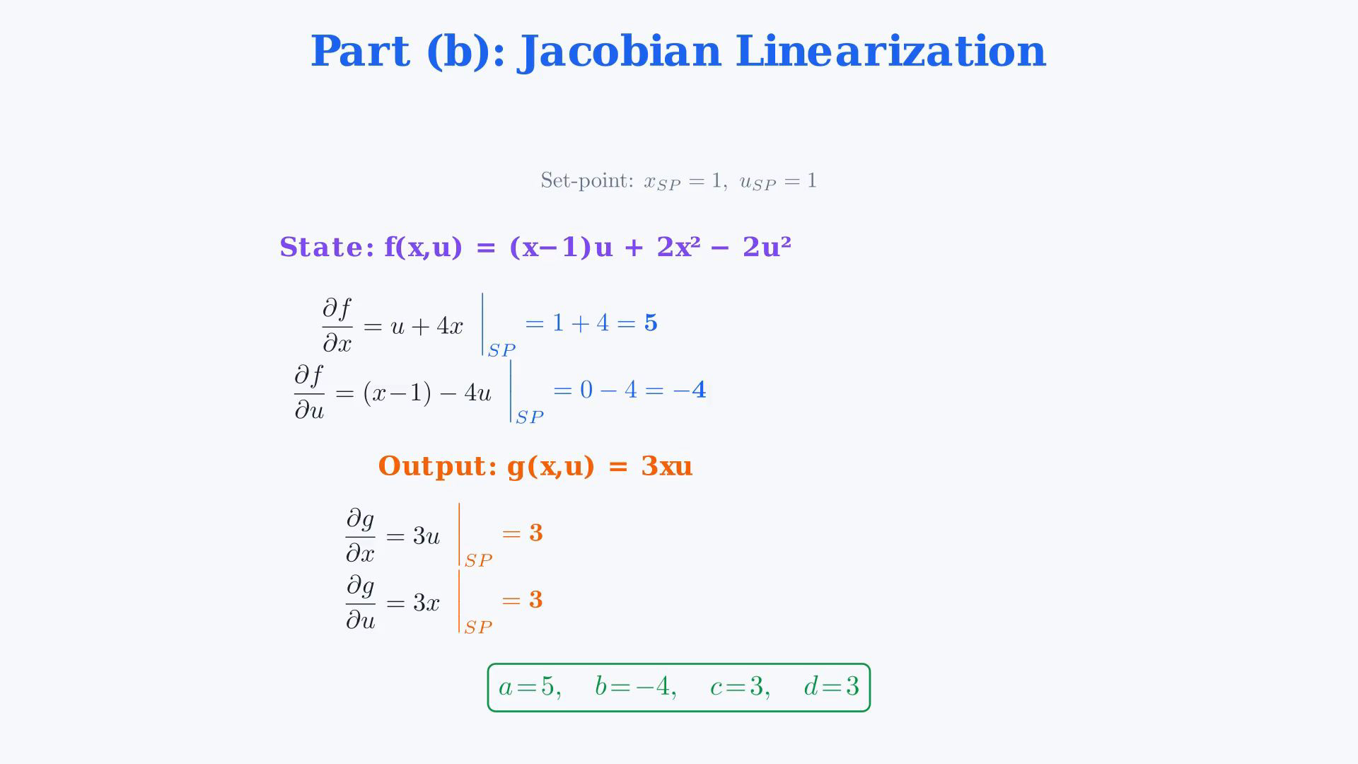
Keep the whole factor (x minus one) multiplied by u. The final model uses deviations from x=1, u=1 and y=3. Its positive state coefficient describes local open-loop instability. Evaluate at the selected point:Find the two state partials and the two output partials.State map:Hold u fixed:State coefficient at the operating point:Hold x fixed:Input coefficient at the operating point:Output map:Hold u fixed:Each of these output partials evaluates to three at the operating point.Hold x fixed:Each of these output partials evaluates to three at the operating point.Narration transcript
Now we linearize at x set-point equals 1, u set-point equals 1. We need the Jacobian, the partial derivatives of f and g. The state function is f of x, u equals the quantity x minus 1 times u, plus 2 x squared, minus 2 u squared. The partial derivative of f with respect to x equals u plus 4 x. At the set-point: 1 plus 4 equals 5. The partial derivative of f with respect to u equals x minus 1, minus 4 u. At the set-point: 0 minus 4 equals negative 4. For the output function g of x, u equals 3 x u. The partial derivative of g with respect to x equals 3 u. At the set-point: 3. The partial derivative of g with respect to u equals 3 x. At the set-point: 3.
4. Write the model for small deviations
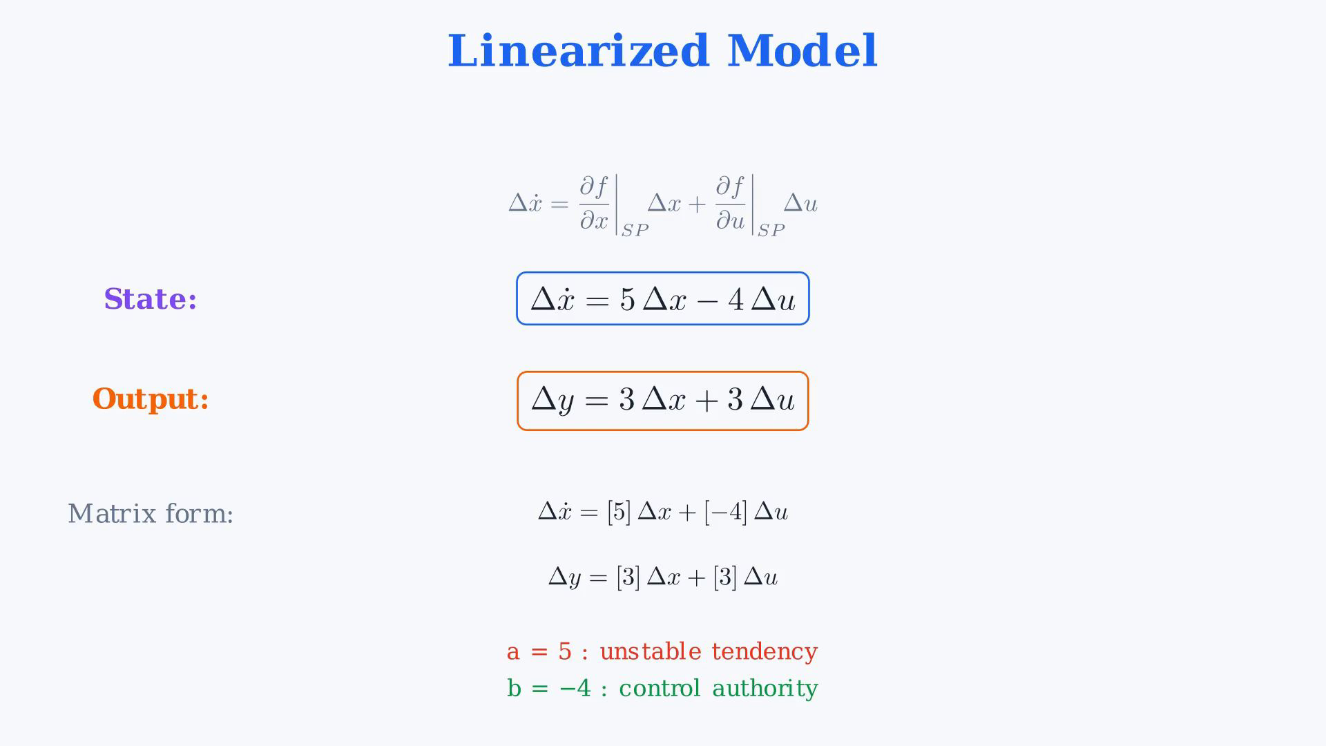
Keep the whole factor (x minus one) multiplied by u. The final model uses deviations from x=1, u=1 and y=3. Its positive state coefficient describes local open-loop instability. First-order state deviation model:First-order output deviation model:Local coefficients:These coefficients describe small deviations near the chosen equilibrium.With the input fixed, the positive state coefficient gives a growing local perturbation.A positive small input perturbation reduces the state derivative at fixed state.Both output sensitivities are three; the input also has a direct output contribution.Output baseline and deviation:Narration transcript
Putting it all together, the linearized state space model is: delta x dot equals 5 delta x minus 4 delta u. delta y equals 3 delta x plus 3 delta u. In matrix notation: the a coefficient is 5, the b coefficient is negative 4, the c coefficient is 3, and the d coefficient is 3. Notice what these numbers tell us about the local behavior near the set-point. A small perturbation in x amplifies x dot by a factor of 5, an unstable tendency. A small perturbation in u decreases x dot by 4, providing control authority. In the output, both state and input perturbations contribute equally with coefficient 3. This is the complete linearized model.
5. Review the local scope and output baseline
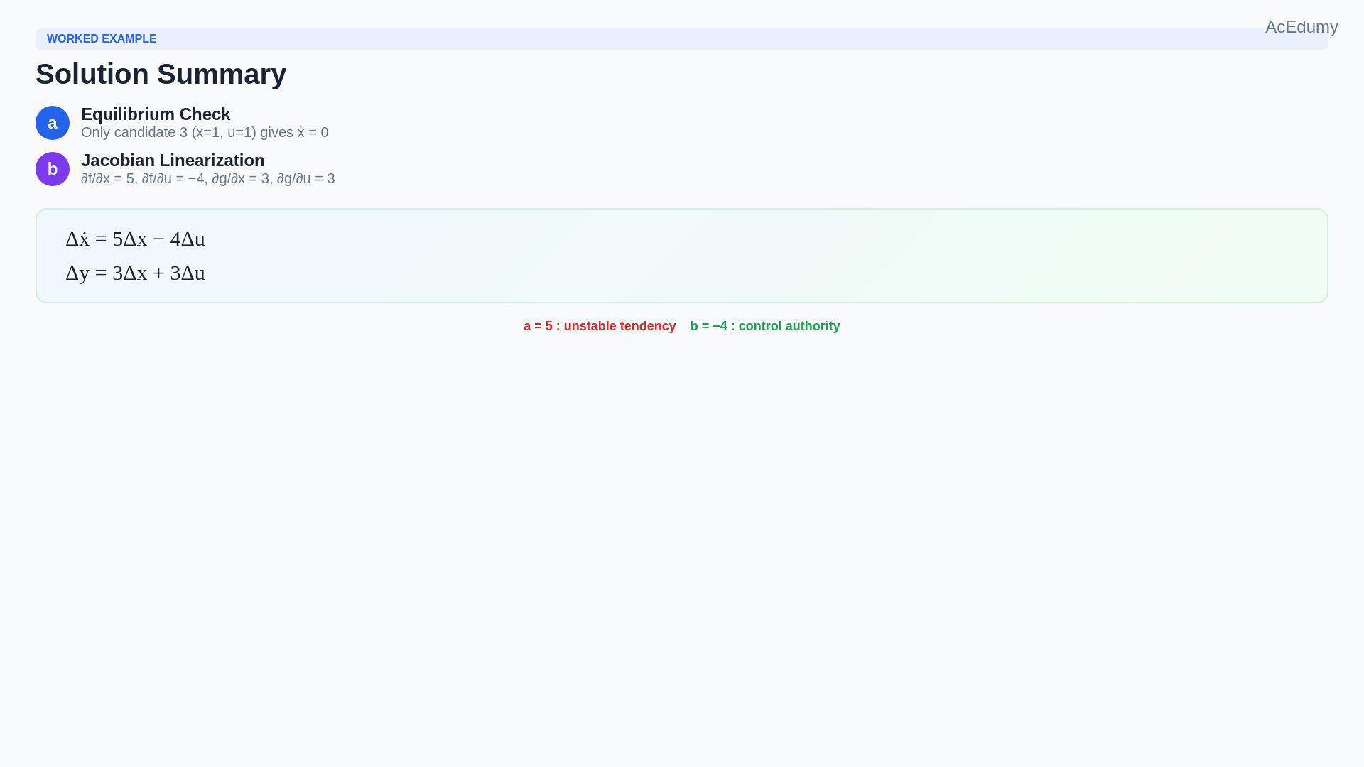
Keep the whole factor (x minus one) multiplied by u. The final model uses deviations from x=1, u=1 and y=3. Its positive state coefficient describes local open-loop instability. Review the calculation.Original state equation:Check equilibrium by substituting each candidate into the state derivative.Selected candidate:Differentiate the state and output maps, then evaluate at the selected point.First-order deviation model:The omitted terms are quadratic; this model is local and the equilibrium is unstable with fixed input.Narration transcript
Let us recap. We had a nonlinear system with x dot equals x minus 1 times u plus 2 x squared minus 2 u squared, and y equals 3 x u. In part a, we checked three candidate set-points by plugging into x dot and requiring it to equal zero. Only candidate 3 with x equals 1 and u equals 1 satisfied the equilibrium condition. In part b, we computed the four partial derivatives of f and g, evaluated them at the set-point, and wrote the linearized model. The result: delta x dot equals 5 delta x minus 4 delta u, and delta y equals 3 delta x plus 3 delta u. Two parts, clean Jacobian linearization, done.
Source video: Control Theory #32 — Set-Point Linearization (Worked Example 9) (5:14)