Control Theory · Plant Modeling: Parallel RC Circuit

#04 Current input, capacitor voltage output, Kirchhoff current law and the differential plant model

Combine Ohm’s law, the capacitor charge relation and Kirchhoff current law to obtain the dynamic parallel RC plant model.

Question

Existing lesson frame showing the plant-model concept, notation analogy or verified differential equations. — The model equation is an algebraic reference for an ideal current source feeding parallel R and C branches. Both elements share the same two nodes; voltage is the signal-node potential minus the reference-node potential, and both passive branch currents leave the signal node. The generic function picture is an analogy: the RC output also depends on input history and initial capacitor voltage.

Assume ideal constant positive resistance and capacitance, an ideal current source, and an unloaded voltage measurement. Define two nodes: a signal node and a reference node. Connect both R and C between those same two nodes. Inject the source current into the signal node; define resistor and capacitor currents from the signal node toward the reference node. Define output voltage as signal-node potential minus reference-node potential. This is a parallel RC topology, so both elements have the same voltage and their branch currents add to the source current. The model-equation frame serves as an algebraic reference for this stated topology. A wire must not bypass either element or join the two nodes directly. The input u is source current i, and output y is capacitor voltage V; voltage is a difference between nodes, not a current arrow or the potential of the grounded node alone. The generic x in the familiar function analogy names an input argument; it does not replace u in the RC derivation or denote a new state variable here. That analogy is not an instantaneous memoryless law for a capacitor: to determine output over time, specify the input history and initial capacitor voltage. The final differential equation supplies the dynamic relationship. For constant C, differentiating charge gives capacitor current; a time-varying C would require the additional product-rule term. The recognized dQ dt and dV dt shorthand refers to derivatives because the narration explicitly introduces differentiation with respect to time and rate of change of charge; the final equation also explicitly says over dt. Treat i as total current and i2 as capacitor branch current, not interchangeable symbols. Charge refers to the plate associated with the positive voltage reference under the passive current convention. The reference node need not be protective earth. Every term in the final equation has current units. The model describes plant dynamics; it does not itself specify a controller or establish tracking performance. No transfer function is derived in this lesson; any later input-output ratio in the Laplace domain requires stating the initial-condition convention.

Written solution and narration transcript(shows the full solution)

Below are all the lines written in the notebook together with the full narration transcript.

1. Introduce plant modeling
The model equation is an algebraic reference for an ideal current source feeding parallel R and C branches. Both elements share the same two nodes; voltage is the signal-node potential minus the reference-node potential, and both passive branch currents leave the signal node. The generic function picture is an analogy: the RC output also depends on input history and initial capacitor voltage.
Introduce Control Theory, Lesson 4.
Model a plant using a parallel RC example.
Narration transcript
Welcome to Control Theory, Lesson 4. Today we'll learn about plant modeling and apply it to a real example, the RC circuit.
2. Define the modeling objective
The model equation is an algebraic reference for an ideal current source feeding parallel R and C branches. Both elements share the same two nodes; voltage is the signal-node potential minus the reference-node potential, and both passive branch currents leave the signal node. The generic function picture is an analogy: the RC output also depends on input history and initial capacitor voltage.
Define plant modeling.
Describe cause and effect between system signals.
Relate the chosen input to the chosen output.
Use the model for prediction and controller design.
Narration transcript
What is plant modeling? It's a mathematical description of the cause-effect relationship between signals in a system. We define how the input affects the output. This mathematical model allows us to design controllers and predict system behavior.
3. State the parallel RC topology
The model equation is an algebraic reference for an ideal current source feeding parallel R and C branches. Both elements share the same two nodes; voltage is the signal-node potential minus the reference-node potential, and both passive branch currents leave the signal node. The generic function picture is an analogy: the RC output also depends on input history and initial capacitor voltage.
Specify the parallel RC topology using two nodes.
An ideal source feeds resistor and capacitor branches connected across the same two nodes.
Measure capacitor voltage relative to the reference node.
Relate source current to capacitor voltage.
Narration transcript
Let's look at our RC circuit. We have a current source providing input current I, a resistor R and a capacitor C in parallel. The output is the voltage V across the capacitor. Our goal is to find the mathematical relationship between input current and output voltage.
4. Map the input and output symbols
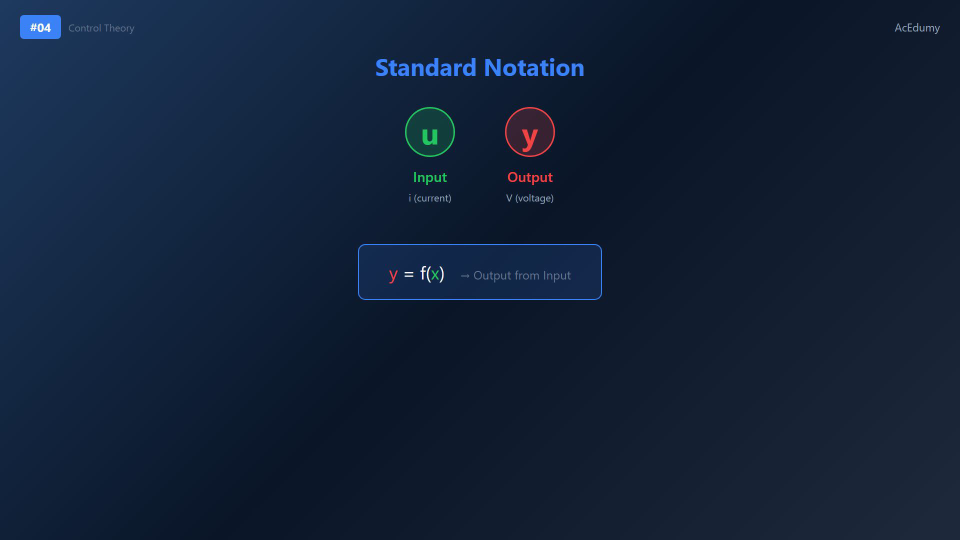
The model equation is an algebraic reference for an ideal current source feeding parallel R and C branches. Both elements share the same two nodes; voltage is the signal-node potential minus the reference-node potential, and both passive branch currents leave the signal node. The generic function picture is an analogy: the RC output also depends on input history and initial capacitor voltage.
Use standard control notation.
Use u for input and y for output.
A generic function analogy uses x as its argument:
$\displaystyle y = f\left(x\right).$
This generic input argument is distinct from a new state variable; dynamic memory still matters.
For this circuit, u is current i and y is voltage V.
Narration transcript
In control engineering, we use standard notation. Input is represented by the letter U and output by the letter Y. Think of it like the function Y equals F of X. The input X gives us the output Y. Here, our input U is the current I and our output Y is the voltage V.
5. Find the resistor current
The model equation is an algebraic reference for an ideal current source feeding parallel R and C branches. Both elements share the same two nodes; voltage is the signal-node potential minus the reference-node potential, and both passive branch currents leave the signal node. The generic function picture is an analogy: the RC output also depends on input history and initial capacitor voltage.
Apply current balance at the signal node:
$\displaystyle i = i₁ + i₂.$
Apply Ohm’s law to the resistor branch.
Resistor branch current:
$\displaystyle i₁ = V/R.$
The shared voltage gives:
$\displaystyle i₁ = V/R.$
Narration transcript
The input current splits into two branches, I1 through the resistor and I2 through the capacitor. For the resistor branch, we use ohms law. The current I1 equals voltage divided by resistance. Since the voltage across the resistor is V, we get I1 equals V over R.
6. Find the capacitor current
The model equation is an algebraic reference for an ideal current source feeding parallel R and C branches. Both elements share the same two nodes; voltage is the signal-node potential minus the reference-node potential, and both passive branch currents leave the signal node. The generic function picture is an analogy: the RC output also depends on input history and initial capacitor voltage.
For constant capacitance:
$\displaystyle Q = C\cdot V.$
Differentiate charge with respect to time:
$\displaystyle Q'\left(t\right) = C\cdot V'\left(t\right).$
Capacitor current is the charge derivative:
$\displaystyle i₂ = C\cdot V'\left(t\right).$
Use this as the capacitor branch relation.
Narration transcript
For the capacitor branch, we start with the charge equation, Q equals C times V. Taking the derivative with respect to time, we get dQ dt equals C times dV dt. Since current is the rate of change of charge, I2 equals C times dV dt. This is the capacitor current equation.
7. Combine the plant model
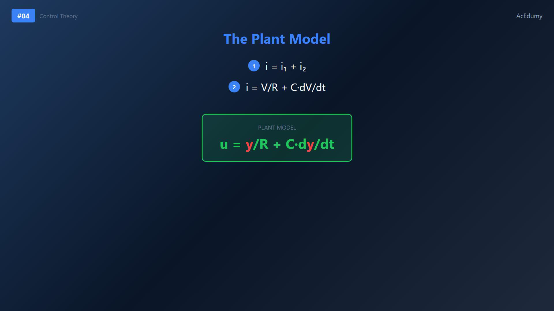
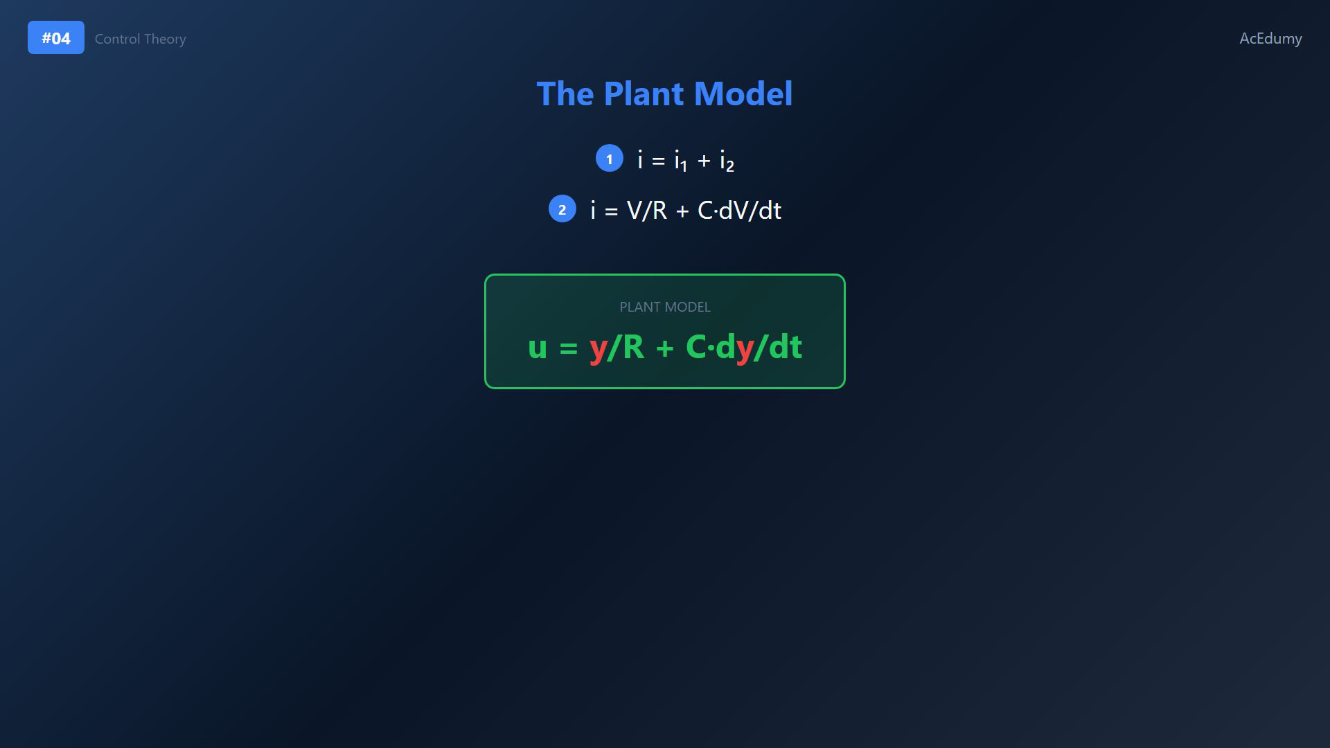
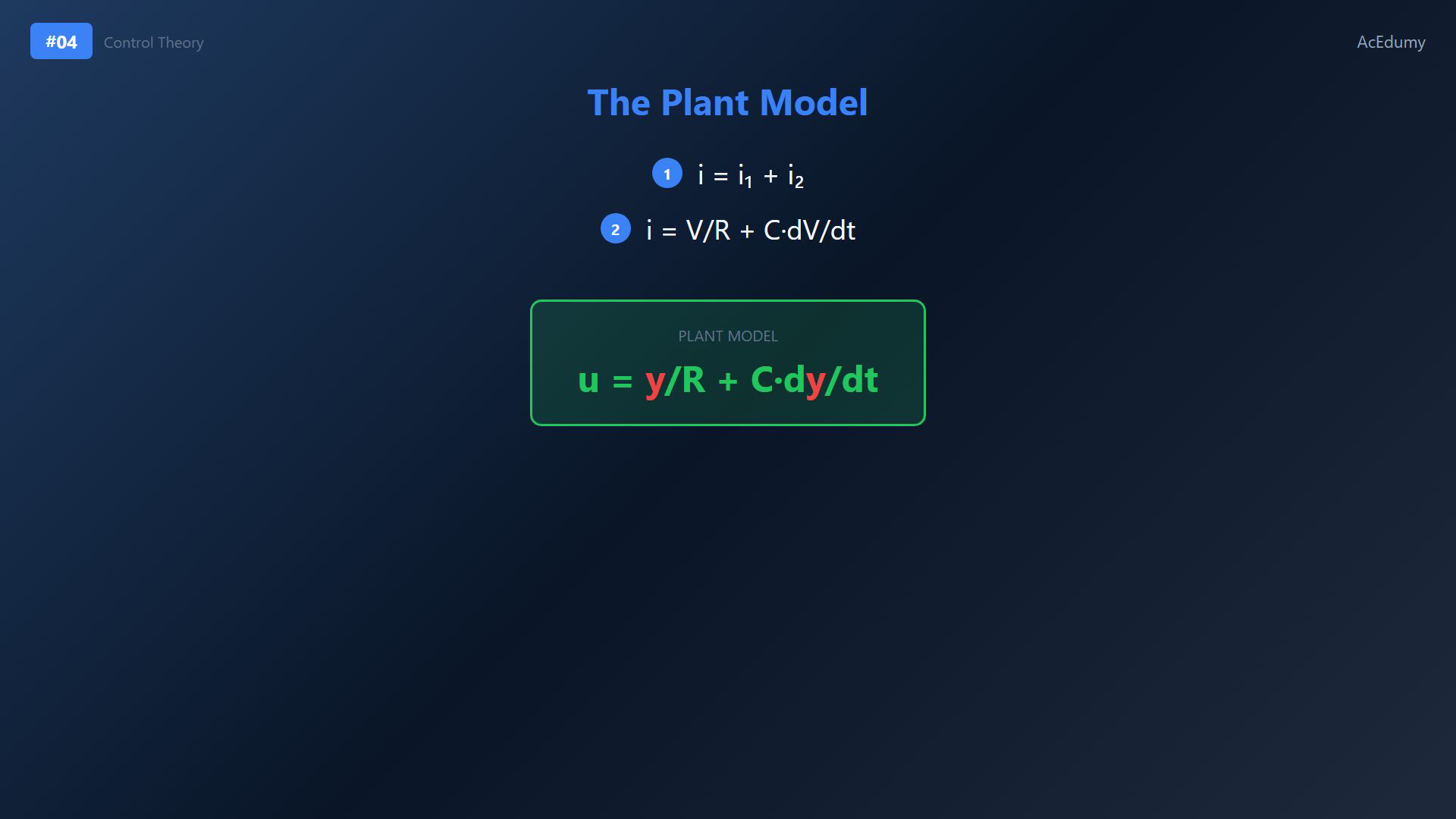
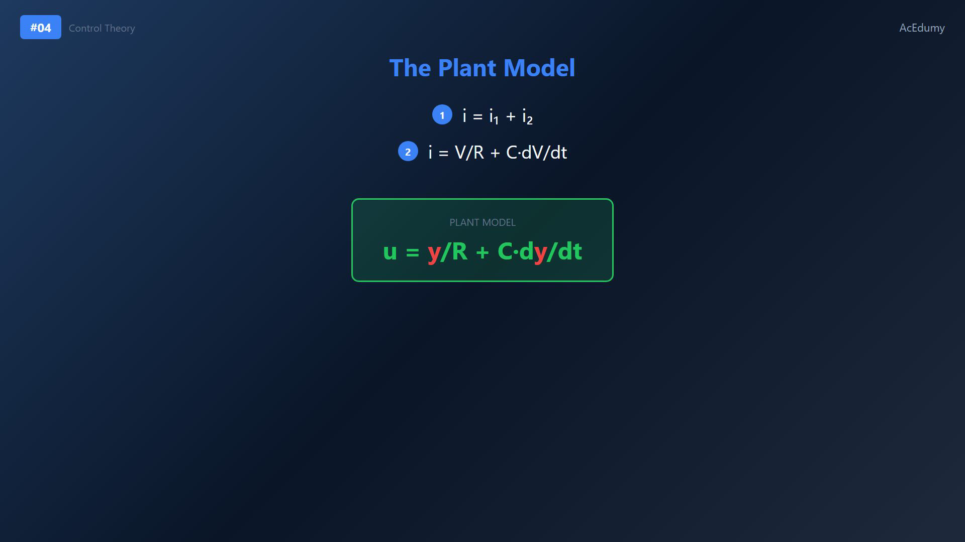
The model equation is an algebraic reference for an ideal current source feeding parallel R and C branches. Both elements share the same two nodes; voltage is the signal-node potential minus the reference-node potential, and both passive branch currents leave the signal node. The generic function picture is an analogy: the RC output also depends on input history and initial capacitor voltage.
Combine the two branch relations.
Kirchhoff current law:
$\displaystyle i = i₁ + i₂.$
Substitute the element relations:
$\displaystyle i =\frac{ V\left(t\right)}{R }+ C\cdot V'\left(t\right).$
Use the chosen input and output symbols:
$\displaystyle u\left(t\right) =\frac{ y\left(t\right)}{R }+ C\cdot y'\left(t\right).$
This differential equation is the plant model.
Narration transcript
Now we combine everything. The total current I equals I1 plus I2. Substituting our expressions, I equals V over R plus C times dV over dt. Using our standard notation with U for input and Y for output, we get U equals Y over R plus C times dy over dt. This is our plant model.
8. Review the dynamic model
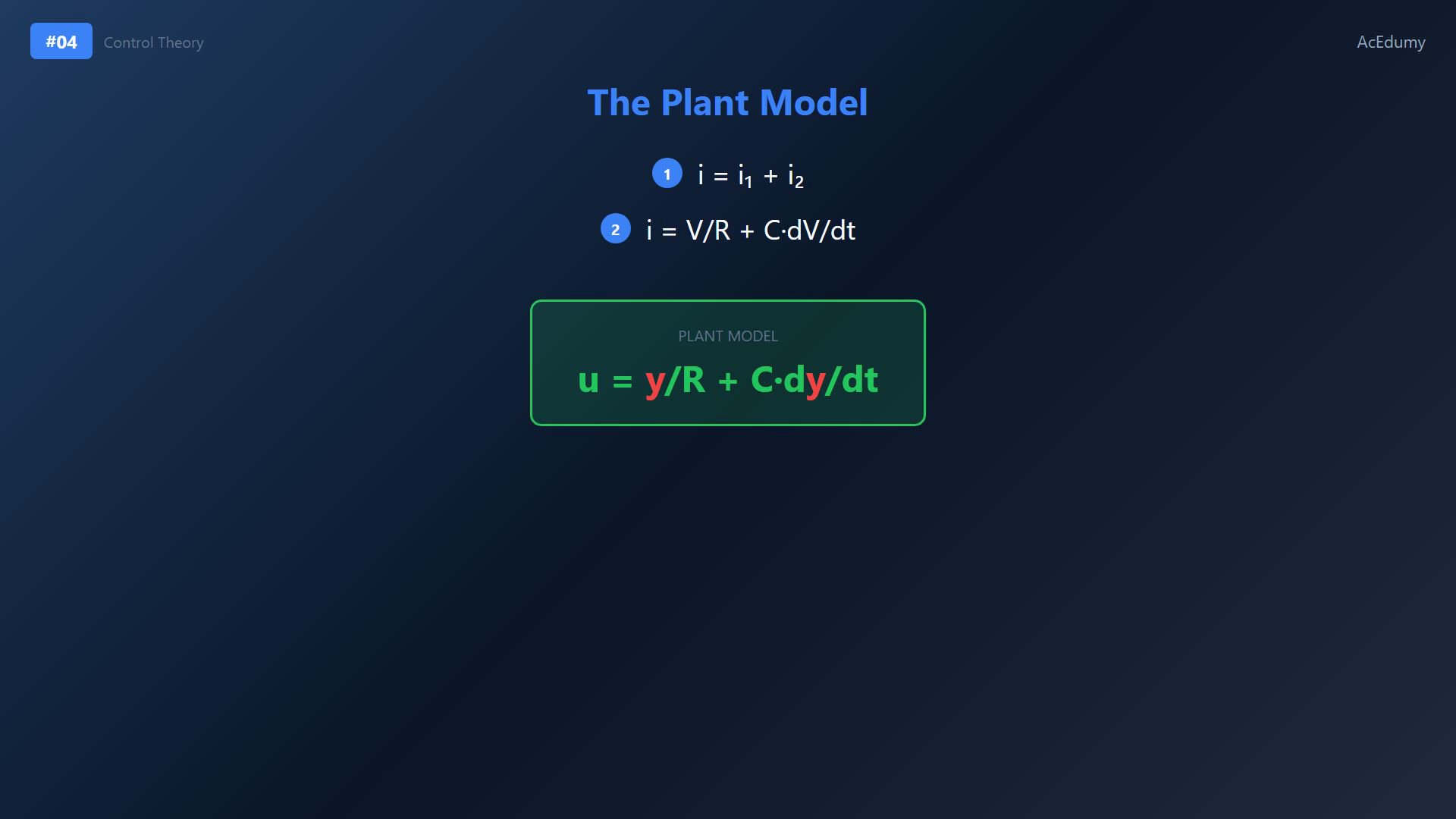
The model equation is an algebraic reference for an ideal current source feeding parallel R and C branches. Both elements share the same two nodes; voltage is the signal-node potential minus the reference-node potential, and both passive branch currents leave the signal node. The generic function picture is an analogy: the RC output also depends on input history and initial capacitor voltage.
Review the parallel RC plant model.
The dynamic relation needs input history and an initial voltage to determine the output.
Next: more systems and block diagrams.
Continue to the next lesson.
Narration transcript
We've successfully modeled our RC circuit plant. The differential equation relates input current to output voltage. In the next lesson, we'll explore more complex systems and block diagrams. See you then.