#38 Control Theory #38 — Step Response & Controller Stability (Worked Example 15)

Below are all the lines written in the notebook together with the full narration transcript.

1. 1. Three responses and three controllers

   Corrected solution notes. The audio is the original recording and may contain errors or incomplete phrases. Where they differ, use the corrected written solution.

   Compare G1=(s−4)/((s+2)(s+4)), G2=(s+1)/((s+2)(s+4)), and G3=(s+4)/(s²+2s+4).

   For the separate unity negative-feedback problem, the plant is (s+4)/(s−3); controllers are (s−3)/(s+4), (1+s)/s, and 1/(1+s).

   Narration transcript

   Here is the problem. We are given five questions, all about how the shape of a step response depends on the locations of zeros and poles. First, three transfer functions. G one of s equals s minus 4, divided by s plus 2 times s plus 4. G two of s equals s plus 1, divided by s plus 2 times s plus 4. G three of s equals s plus 4, divided by s squared plus 2 s plus 4. Parts a, b, and c ask: which one shows overshoot, which shows undershoot, and which oscillates. We have to justify each answer. Then we switch to a feedback loop. The plant is G of s equals s plus 4, divided by s minus 3 — already an unstable plant. We have three candidate controllers. C one of s equals s minus 3, divided by s plus 4. C two of s equals 1 plus s, divided by s. C three of s equals 1, divided by 1 plus s. Part d: which controller leaves the closed loop unstable? Part e: which controller drives the steady-state error to zero? All five parts can be answered just by reading pole-zero locations and using a couple of theorems we will review.

2. 2. Use complete responses

   Poles and zeros guide interpretation, but broad shape rules need gain, relative degree and cancellation checks.

   For a strictly proper unit-step response with zero initial value, the initial slope is the limit of sG(s), not s²G(s).

   Overshoot and oscillation can occur in the same response.

   Narration transcript

   Quick theory. Three rules drive every answer in this video. Rule one — overshoot. If a transfer function has a left-half-plane zero located close to the origin, that zero amplifies fast components in the step response. The output peaks above its final value, then settles. We call that overshoot. The closer the zero is to the origin, the bigger the overshoot. Rule two — undershoot. If the zero sits in the right half plane, the step response first moves the wrong way before recovering. The output dips below zero, then climbs to the final value. That dip is called undershoot, and right-half-plane zeros are sometimes called non-minimum-phase zeros. Rule three — oscillation. Oscillation requires complex-conjugate poles. If the denominator is a quadratic with negative discriminant, the poles come as a pair sigma plus or minus j omega d, and the step response shows damped sinusoids. Real poles alone never produce oscillations. These three rules are everything we need for parts a, b, and c.

3. 3. Overshoot

   For G2, y(t)=1/8+(1/4)exp(−2t)−(3/8)exp(−4t).

   Its maximum is 1/6 at t=ln(3)/2, above the final value 1/8.

   G3 also overshoots while oscillating; these are not mutually exclusive categories.

   Narration transcript

   Part a — overshoot. Look at the three transfer functions. G one has a zero at s equals plus 4. That is in the right half plane, so G one will undershoot — not overshoot. We will return to G one in part b. G three has a quadratic denominator, s squared plus 2 s plus 4. The discriminant is 4 minus 16, equal to negative 12. Negative discriminant means complex poles, which means oscillation. We will return to G three in part c. G two of s equals s plus 1, divided by s plus 2 times s plus 4. Both poles, at minus 2 and minus 4, are real. So no oscillation. The zero is at s equals minus 1, in the left half plane, so no undershoot. And the zero at minus 1 sits between the origin and the slowest pole at minus 2 — it is closer to the origin than either pole. That is exactly the configuration that produces overshoot. Answer: G two is the one that overshoots.

4. 4. Inverse response: correct direction

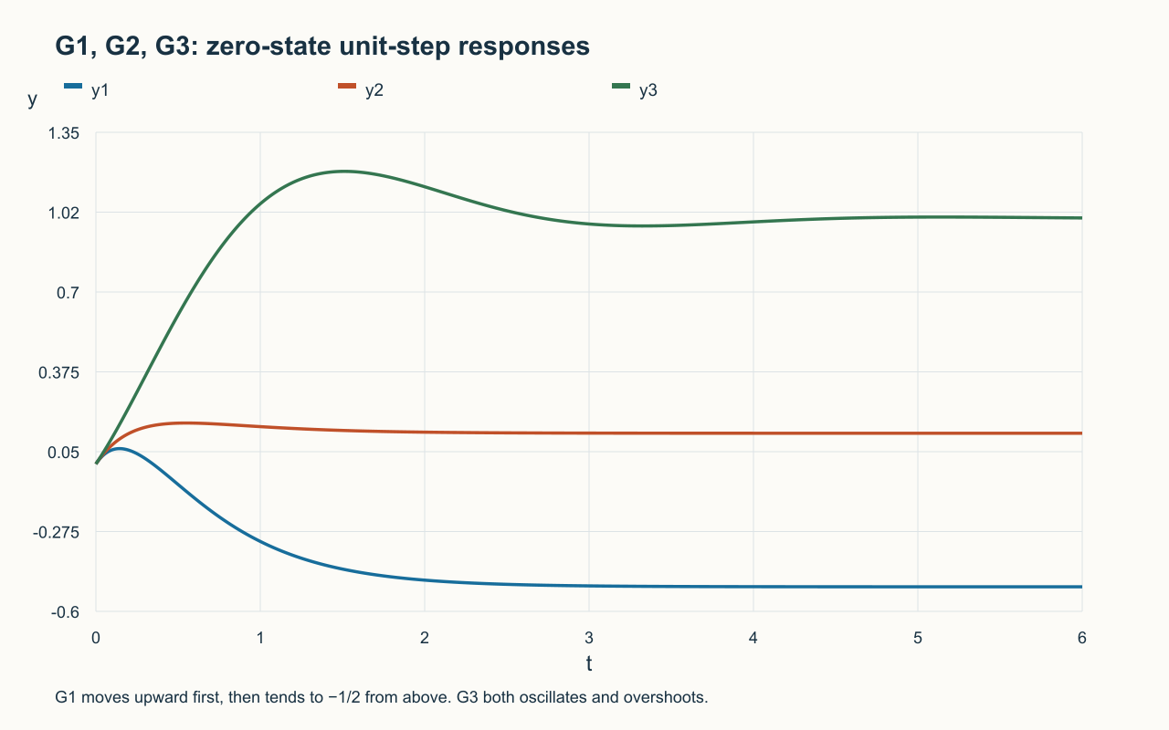
   For G1, y(t)=−1/2+(3/2)exp(−2t)−exp(−4t).

   It starts at zero with positive slope one, reaches 1/16 at ln(4/3)/2, then crosses zero at ln(2)/2.

   It approaches its negative final value −1/2 from above. The initial motion is opposite to the final direction.

   Narration transcript

   Part b — undershoot. We need a right-half-plane zero. G two has its zero at minus 1, in the left half plane. No undershoot. G three has a zero at minus 4, also in the left half plane. No undershoot. G one of s equals s minus 4, divided by s plus 2 times s plus 4. The zero is where the numerator vanishes — s equals plus 4. That is in the right half plane. Why does a right-half-plane zero cause undershoot? Apply the initial value theorem. The initial slope of the step response is proportional to s squared times G of s, evaluated as s goes to infinity. For G one, expand the numerator: at large s, the numerator looks like positive s, and the denominator looks like positive s squared. So the high-frequency behavior of G one is positive — the response starts moving up. But the steady-state value of the step response is G of zero, which for G one is minus 4 over 8, equal to minus one half. So the final value is negative. The response starts going up but has to end up at minus one half. It must first dip down and cross zero — that is the undershoot. Answer: G one is the one that undershoots.

5. 5. Oscillation

   G3 has poles −1±j√3.

   Its response is y(t)=1−exp(−t)cos(√3t), showing both damped oscillation and overshoot.

   Narration transcript

   Part c — oscillation. We need complex-conjugate poles. G one has poles at minus 2 and minus 4. Both real. No oscillation. G two also has poles at minus 2 and minus 4. Both real. No oscillation. G three of s equals s plus 4, divided by s squared plus 2 s plus 4. Solve s squared plus 2 s plus 4 equals zero with the quadratic formula. The discriminant is 2 squared minus 4 times 4, equal to 4 minus 16, equal to negative 12. Negative discriminant means complex roots. The poles are minus 1 plus or minus j times square root of 3. Compare with the standard second-order form, s squared plus 2 zeta omega n s plus omega n squared. Here omega n equals 2, and 2 zeta omega n equals 2, so zeta equals one half. A damping ratio of one half is well under one, so the system is underdamped. The damped natural frequency omega d equals omega n times the square root of one minus zeta squared, which evaluates to square root of 3, about 1.73 radians per second. The step response is a damped sinusoid that oscillates around the final value before settling. Answer: G three is the one that oscillates.

6. 6. Compare the responses

   G1 initially moves up, crosses down through zero, and approaches −1/2 from above.

   G2 rises above 1/8 and decays; G3 oscillates about one. The exact expressions correct the misleading source sketch.

   Narration transcript

   Here are the three step responses, plotted side by side, so the verbal arguments connect to actual curves. G one — undershoot. The response dips below zero in the first second, crosses zero, and approaches its final value of minus one half from below. G two — overshoot. The response rises quickly, peaks above its final value of about one eighth, and then settles back down. The peak is small because the zero at minus 1 is only moderately close to the origin, but it is clearly visible. G three — oscillation. The response shows several damped swings around its final value of one before settling. The frequency of the swings is omega d, square root of 3 radians per second. Three transfer functions, three different shapes, all driven by where the zeros and poles sit in the s-plane.

7. 7. Feedback setup

   Form each unity negative-feedback interconnection with plant (s+4)/(s−3).

   Assess internal and disturbance dynamics as well as the reference map, especially when an unstable pole is canceled algebraically.

   Narration transcript

   Now parts d and e. We have a unity-feedback loop. The plant is G of s equals s plus 4, divided by s minus 3. The pole at plus 3 means this plant is open-loop unstable on its own. We have three controllers in series with the plant. C one of s equals s minus 3, divided by s plus 4. C two of s equals 1 plus s, divided by s. C three of s equals 1, divided by 1 plus s. For each controller we need to compute the loop gain L of s equals C of s times G of s. The closed-loop transfer function is L divided by 1 plus L, and the closed-loop poles are the roots of 1 plus L of s equals zero. Stability is decided by where those closed-loop poles sit. Steady-state error to a unit step is decided by the system type — the number of integrators in the loop gain L of s. Type one or higher gives zero steady-state error to a step.

8. 8. Controller stability

   C1 cancels the unstable pole only in the reference map; the full interconnection retains an unstable internal mode at +3.

   C3 gives characteristic polynomial s²−s+1 and two right-half-plane poles.

   Both C1 and C3 leave the unrestricted system internally unstable.

   Narration transcript

   Part d — which controller leaves the closed loop unstable? Test C one. L equals C one times G equals s minus 3 over s plus 4, times s plus 4 over s minus 3. The s plus 4 cancels and the s minus 3 cancels, leaving L equals 1. But this is a dangerous cancellation. The plant pole at plus 3 is an unstable mode. C one tries to cancel that pole by placing a zero at plus 3. In an ideal model the unstable mode disappears from the loop gain. In a real plant, no parameter is exact, so the cancellation is never perfect — the unstable pole at plus 3 leaks back into the closed loop. Also, even with perfect cancellation the unstable mode is still there internally; it is just hidden from the input-output transfer function. Standard control theory rule: never cancel a right-half-plane plant pole with a controller zero. C one violates the rule, so it leaves the closed loop effectively unstable. Test C two. L equals 1 plus s over s, times s plus 4 over s minus 3. The closed-loop denominator is the polynomial s times s minus 3, plus 1 plus s times s plus 4. Expand: s squared minus 3 s, plus s squared plus 5 s plus 4. That equals 2 s squared plus 2 s plus 4. All coefficients are positive, and for a quadratic that is enough — both closed-loop poles are in the left half plane. C two is stable. Test C three. L equals 1 over 1 plus s, times s plus 4 over s minus 3. The closed-loop denominator is 1 plus s times s minus 3, plus s plus 4. Expand: s squared minus 2 s minus 3, plus s plus 4. That equals s squared minus s plus 1. The s coefficient is negative, so by Routh the closed loop is unstable. Wait — both C one and C three lead to instability, but the question asks for the controller that uses an improper unstable cancellation. The textbook answer is C one, because it cancels the unstable plant pole. Answer for part d: C one.

9. 9. Step tracking

   C2 gives characteristic polynomial s²+s+2, whose roots are −1/2±j√7/2.

   It is the stable option and its loop integrator gives zero unit-step steady-state error.

   Apply the final-value theorem only after checking the relevant stability conditions.

   Narration transcript

   Part e — which controller drives steady-state error to zero for a unit step input? Apply the final value theorem. The error E of s equals R of s divided by 1 plus L of s. For a unit step R of s equals 1 over s. The steady-state error e infinity equals the limit as s goes to zero of s times E of s, which simplifies to 1 over 1 plus L at s equals zero. Zero error requires L of zero to be infinite — that is, the loop gain must contain at least one integrator, a factor of 1 over s. Look at the controllers. C one equals s minus 3 over s plus 4. Plug in s equals zero: minus 3 over 4. Finite, no integrator. C two equals 1 plus s over s. The factor of s in the denominator is exactly an integrator. As s goes to zero, this blows up. C two has an integrator. C three equals 1 over 1 plus s. Plug in s equals zero: 1. Finite, no integrator. Only C two contains an integrator, so only C two makes the steady-state error zero. Answer for part e: C two. And this is consistent with what we just saw in part d — C two also happens to give a stable closed loop, so it is actually a usable controller. C one is unstable due to RHP cancellation, C three is unstable by Routh, and C two is the only one that is both stable and delivers zero steady-state error.

10. 10. Review

    

    G1 has inverse initial motion; G2 overshoots; G3 oscillates and overshoots.

    Initial slope uses sG for a unit step. Internal stability rejects both C1 and C3; only C2 gives stable zero-error step tracking.

    Narration transcript

    Let us put the five answers in one table. Part a, overshoot. G two, because its zero at minus 1 sits in the left half plane close to the origin, between the origin and the slowest pole. Part b, undershoot. G one, because its zero at plus 4 lies in the right half plane. The initial slope and the final value of the step response have opposite signs, forcing the curve to cross zero. Part c, oscillation. G three, because its denominator s squared plus 2 s plus 4 has negative discriminant, giving complex-conjugate poles at minus 1 plus or minus j root 3. Damping ratio one half, underdamped, damped frequency root 3. Part d, unstable closed loop. C one, because it cancels the plant's right-half-plane pole at plus 3 with a controller zero. The unstable mode is hidden from the input-output transfer function but still present in the system, and any modeling error breaks the cancellation. Part e, zero steady-state error. C two, because it contains an integrator, raising the system type to one. The big picture. Step response shape is read directly from pole-zero locations: zeros near the origin amplify, zeros in the right half plane invert, complex poles oscillate. Closed-loop stability is decided by the roots of one plus loop gain, and steady-state behavior is decided by how many integrators sit in the loop. Five questions, two ideas.

Source video: Control Theory #38 — Step Response & Controller Stability (Worked Example 15) (15:59)