Control Theory · Parametric stability problem
#42 Control Theory #42 — Routh-Hurwitz Parametric Stability (Worked Example 19)
Corrected solution notes. The audio is the original recording and may contain errors or incomplete phrases. Where they differ, use the corrected written solution.
Question
Corrected solution notes. The audio is the original recording and may contain errors or incomplete phrases. Where they differ, use the corrected written solution. Control Theory #42 — Routh-Hurwitz Parametric Stability (Worked Example 19)
Written solution and narration transcript(shows the full solution)
Below are all the lines written in the notebook together with the full narration transcript.
1. Parametric stability problem
Corrected solution notes. The audio is the original recording and may contain errors or incomplete phrases. Where they differ, use the corrected written solution.G(s)=(s+3)/(3s⁴+3Ks³+4s²+Ks+1/3).Determine strict BIBO stability of this proper reduced transfer function. Any cancellation must be checked; the only possible cancellation here removes a stable pole at −3 and does not change the stable range.Narration transcript
Here is the problem. We are handed a transfer function G of s equals s plus three, divided by three s to the fourth, plus three K s cubed, plus four s squared, plus K s, plus one third. Inside the denominator sits a free parameter K. Our job — find every value of K for which this transfer function is stable. Stability of an isolated transfer function means one thing only — every pole, every root of the denominator polynomial, must sit strictly in the open left half plane. The numerator does not matter for stability. The zero at minus three plays no role here. So the question reduces to one polynomial — three s to the fourth, plus three K s cubed, plus four s squared, plus K s, plus one third. For which K does every root of this fourth-order polynomial sit in the open left half plane? Solving a fourth-order polynomial by hand for arbitrary K is brutal — the roots are messy functions of K. We need a smarter route. That route is Routh-Hurwitz.
2. Routh method
Positive coefficients are necessary for a real polynomial to be strictly Hurwitz after choosing a positive leading coefficient.A zero row or zero pivot requires special treatment. Failure of strict stability does not by itself prove exponential divergence for every input.Narration transcript
The strategy. Routh-Hurwitz gives stability without ever computing a single root. It works in two stages. Stage one — the necessary condition. For every root to sit in the open left half plane, every coefficient of the polynomial must be present and share the same sign. If any coefficient is zero, or if the signs disagree, the system is already unstable. Done — we can stop. Stage two — the Routh table. Build a table from the polynomial coefficients. Compute its first column. Stability is equivalent to the statement that every entry in the first column shares the same sign — no sign changes top to bottom. When the polynomial has a parameter like K inside, the entries become expressions in K. Each entry that depends on K becomes an inequality. The system of inequalities, taken together, gives the K range for stability. We will run both stages — necessary condition first, then the full Routh table — and combine the constraints at the end.
3. Necessary condition
With coefficients 3, 3K, 4, K, 1/3, strict Hurwitz stability requires K>0.At K=0, two coefficients vanish. Examine that boundary separately rather than substituting zero into divisions by K.Narration transcript
Stage one — the necessary condition. List the coefficients of the denominator, in order. Three, three K, four, K, one third. Two of them carry the parameter — three K and K. The other three are fixed positive numbers. For the necessary condition to hold, every coefficient must be strictly positive — same sign, no zeros. Three is positive. Always. Four is positive. Always. One third is positive. Always. Three K is positive when K is positive. K is positive when K is positive. Combine. The necessary condition fires once on a single inequality — K greater than zero. If K is zero or negative, the system is already unstable, no further work needed. K greater than zero is necessary. Whether it is also sufficient — that is what the Routh table will decide.
4. First two rows
The s⁴ row is [3, 4, 1/3].The s³ row is [3K, K, 0].For nonzero pivots, each new row is computed from the preceding two rows using the signed Routh formula.Narration transcript
Stage two — the Routh table. Lay out the first two rows directly from the coefficients. The s to the fourth row collects every other coefficient starting from the leading term — three, four, one third. The s cubed row collects the remaining coefficients — three K, K, and a trailing zero to fill the row. These two rows are written. The remaining three rows must be computed. The recipe is the same for every cell. Take a two-by-two block — the leading column from the previous two rows on the left, and the column above and to the right of the cell on the right. Take the determinant of that block. Divide by the leading element of the row immediately above. Move on to the next column. The structure is mechanical. Compute s squared row — two cells. Compute s to the one row — one cell. Compute s to the zero row — one cell. Five cells total. Then read the first column.
5. The s² row
For K≠0, its first entry is (12K−3K)/(3K)=3.Its second entry is K/(3K)=1/3. Thus the row is [3, 1/3, 0].Narration transcript
The s squared row. Two cells to compute, both built from the first two rows. First cell — call it b one. Take the two-by-two block. Top row, three and four. Bottom row, three K and K. Cross multiply. Three K times four is twelve K. Three times K is three K. Subtract. Twelve K minus three K is nine K. Divide by the leading element of the row above — three K. Nine K divided by three K is three. b one equals three. The K cancels. The cell is a fixed positive number, with no dependence on K. Second cell — call it b two. Top row, three and one third. Bottom row, three K and zero. Cross multiply. Three K times one third is K. Three times zero is zero. Subtract. K minus zero is K. Divide by three K. K divided by three K is one third. b two equals one third. Again the K cancels — another fixed positive number. The s squared row is now three, one third, zero. Both nontrivial cells are positive constants. The K-dependence has bubbled away.
6. The last two rows
The s¹ entry is (3K−K)/3=2K/3.The s⁰ entry is 1/3. The generic calculation applies for K≠0.Narration transcript
The s to the one row. One cell, call it c one. Take the two-by-two block from the previous two rows. Top row, three K and K. Bottom row, three and one third. Cross multiply. Three times K is three K. Three K times one third is K. Subtract. Three K minus K is two K. Divide by the leading element of the row above — three. c one equals two K divided by three, or equivalently two K over three. Here the K survives. The cell depends on K. The s to the zero row. One cell, call it d one. Take the block. Top row, three and one third. Bottom row, two K over three and zero. Cross multiply. Two K over three times one third is two K over nine. Three times zero is zero. Subtract. Two K over nine minus zero is two K over nine. Divide by the leading element of the row above — two K over three. Two K over nine divided by two K over three. The two K cancels. What remains is one over nine, divided by one over three, which equals three over nine, which equals one third. d one equals one third. The K cancels again. The bottom of the table is a fixed positive constant.
7. Strict range and boundary
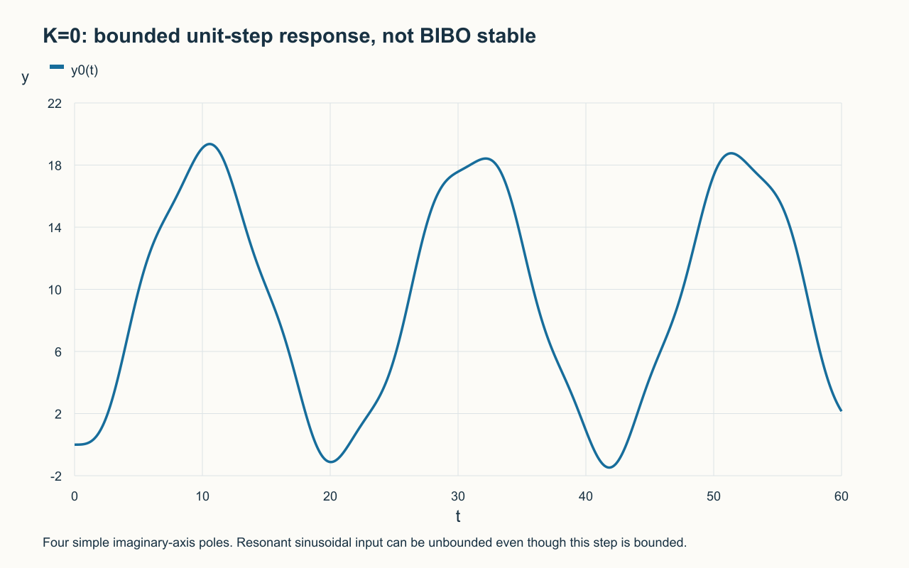
The first column is [3, 3K, 3, 2K/3, 1/3]. For K>0 there are no sign changes; for K<0 there are four.At K=0 the denominator is 3(s²+a)(s²+b), with a=(2−√3)/3 and b=(2+√3)/3.Its four poles are simple imaginary-axis poles: ±j√a and ±j√b. None is in the open right half-plane.Narration transcript
The first column of the Routh table is now complete. From top to bottom — three, three K, three, two K over three, one third. Stability requires every entry to share the same sign — and since the leading entry is positive, every entry must be strictly positive. Walk down the column. Three is positive. No constraint on K. Three K is positive when K is positive. One inequality. Three is positive. No constraint on K. Two K over three is positive when K is positive. Same inequality, repeated. One third is positive. No constraint on K. Two of the five entries depend on K, and both demand the same thing — K greater than zero. Combine with the necessary condition from stage one — also K greater than zero. The two stages agree. Final answer. The transfer function G of s is stable for every K greater than zero, and unstable for every K less than or equal to zero. A clean parametric stability boundary at K equals zero. Above the boundary, all four poles sit in the open left half plane. At or below the boundary, at least one pole crosses into the right half plane and the system blows up.
8. Correct the response claim
At K=0 the zero-state unit-step response is a bounded sum of a constant, sines and cosines. It does not settle.The transfer function is nevertheless not BIBO stable: a bounded sinusoid at a pole frequency produces resonant unbounded growth.For K<0 the uncanceled right-half-plane modes are unstable; for K>0 the system is strictly stable.Narration transcript
Verification. We have a clean answer — K greater than zero for stability. Let us spot-check by plugging in numbers and looking at the actual step response. Top left panel — K equals two. Comfortably inside the stable region. The step response oscillates briefly, then settles to a finite value. Bounded. Stable. Matches the theory. Top right panel — K equals zero point one. Still positive, but close to the boundary. The response rings longer — the small K starves the damping — but it still settles. Stable, just barely. The boundary is reached gracefully from above. Bottom left panel — K equals zero. Exactly on the boundary. The necessary condition fails — one coefficient is now zero. The response drifts and oscillates without bound. Marginally unstable, as predicted. Bottom right panel — K equals minus zero point five. Below the boundary. The denominator now has a coefficient of the wrong sign, and the response explodes — the curve runs off the chart. Strongly unstable, as predicted. Four data points, four matches. Routh-Hurwitz delivered the right answer without ever computing a single pole.
9. Review
Corrected mathematical reference; use with the written derivation. Strict BIBO stability holds exactly for K>0.The K=0 boundary is marginal in a minimal unforced realization and fails BIBO stability, while its particular step response remains bounded.Distinguish asymptotic stability, BIBO stability and the behavior of a single chosen input.Narration transcript
Summary. The problem. G of s equals s plus three over three s to the fourth, plus three K s cubed, plus four s squared, plus K s, plus one third. For which K is the transfer function stable? The method. Routh-Hurwitz. Necessary condition first, then the full Routh table. The Routh first column. Three, three K, three, two K over three, one third. The constraints. Only two entries depend on K. Both demand K greater than zero. The answer. G of s is stable if and only if K is greater than zero. The big idea. When a transfer function carries a free parameter inside its denominator, the Routh table converts the stability question into a system of inequalities in that parameter. Solve the inequalities — get the stable range. No root finding required. The same method scales — it works for any parameter, any number of coefficients, any order of polynomial. The parametric stability boundary is the most useful tool a control engineer carries into design.
Source video: Control Theory #42 — Routh-Hurwitz Parametric Stability (Worked Example 19) (11:53)