Control Theory · Drawing the RC Block Diagram from Its Differential Equation

#07 Convert the parallel RC plant equation into an integrator realization with an internal return path

Identify the current input and voltage output, preserve initial conditions, and realize the RC model using a signed sum, constant gains and an integrator.

Question

Existing lesson frame showing the RC equation, drawing procedure or an intermediate signal-flow construction. — The compact integral equation is an algebraic reference with its initial-value term suppressed. Intermediate construction frames show only the blocks introduced so far. The gain frame places 1/C before integration; the narration first describes it after integration. These are equivalent for constant C and matched initial values. Equation reference cards accompany the return-path, complete, combined and comparison explanations.

Use the ideal parallel RC model with constant positive resistance R and capacitance C. Input u is the applied current and output y is the capacitor voltage; prime notation means the time derivative. The equation C times the derivative of y plus y/R equals u describes the plant. The four steps construct an integrator realization for this model; they are not a prohibition on differentiator blocks in every possible diagram. Integrating from a common initial time requires the initial voltage. The source uses compact indefinite-integral notation and suppresses its constant; with lower limit zero its displayed form assumes zero initial voltage. For arbitrary initial voltage y0, add y0 to the integral expression for y. Do not infer that integration erases the initial state. Combine the two integrals by linearity with identical limits and constant R and C; having the same degree alone is not sufficient. The inner operation subtracts the product (1/R) times y from u. The brief spoken ry shorthand refers to that product, repeatedly stated explicitly and shown in the preceding equation; it does not mean 1/(R times y). Both summing inputs therefore have current units. Multiplication by 1/C produces the rate of change of voltage, and integration yields voltage. Place the input plus and return-path minus clearly at their respective junction inputs, and draw connected signal arrows. These are signal-flow diagrams, not physical circuit wiring. Early frames are partial construction stages, with the full return path still to be supplied. Read the full realization as: u enters positively, y passes through gain 1/R and enters negatively, the resulting difference passes through gain 1/C and an integrator, and its output is y. The gain-stage narration places 1/C after the integrator, whereas its picture and subsequent complete explanation place it before. For constant C both orders agree when their internal states are matched: the gain-before integrator starts at y0; the integrate-before-gain route starts its integrator at C times y0. Do not move a time-varying capacitance coefficient through an integral. The combined block includes this same gain, integration and initial-state convention. Changing the forward-path grouping must retain the return gain 1/R and negative sign. The clean equation cards are algebraic references for these operations, not complete block drawings. This return path is an internal realization of a passive RC plant; no separate controller, reference command or sensor has been designed here. The time constant is R times C. The phrase capacitance affects the gain refers to the internal 1/C coefficient and transient response: the steady-state voltage/current gain is R, independent of C. The model is first order and needs one initial voltage. No tracking or regulation guarantee follows from drawing this internal loop.

Written solution and narration transcript(shows the full solution)

Below are all the lines written in the notebook together with the full narration transcript.

1. Introduce the RC realization
The compact integral equation is an algebraic reference with its initial-value term suppressed. Intermediate construction frames show only the blocks introduced so far. The gain frame places 1/C before integration; the narration first describes it after integration. These are equivalent for constant C and matched initial values. Equation reference cards accompany the return-path, complete, combined and comparison explanations.
Introduce Control Theory, Lesson 7.
Draw a block diagram from a differential equation.
Use the parallel RC model from Lesson 4.
Narration transcript
Welcome to lesson 7 of Control Theory. Today we'll draw a block diagram from a real differential equation. We'll use the RC circuit model from lesson 4 as our example.
2. Recall the RC model
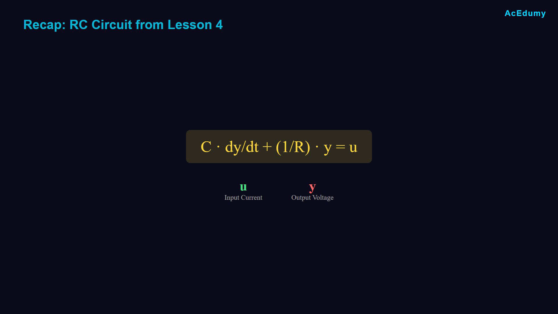
The compact integral equation is an algebraic reference with its initial-value term suppressed. Intermediate construction frames show only the blocks introduced so far. The gain frame places 1/C before integration; the narration first describes it after integration. These are equivalent for constant C and matched initial values. Equation reference cards accompany the return-path, complete, combined and comparison explanations.
Recall the RC plant model.
Current balance:
$\displaystyle C\cdot y'\left(t\right) + \left(\frac{1}{R}\right)\cdot y\left(t\right) = u\left(t\right).$
Identify u as current input and y as voltage output.
Convert this first-order model to a block diagram.
Narration transcript
Let's recall the RC circuit equation from lesson 4. We found that C times dy dt plus 1 over r times y equals u. Here u is the input current and y is the output voltage. Now let's convert this to a block diagram.
3. State the drawing procedure
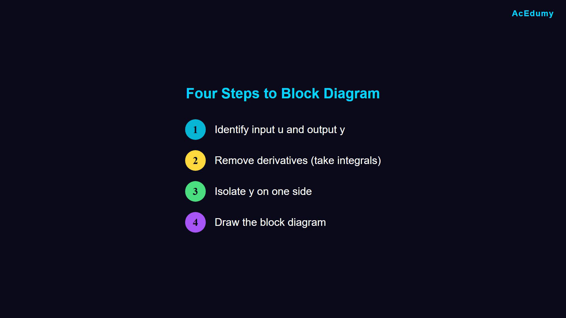
The compact integral equation is an algebraic reference with its initial-value term suppressed. Intermediate construction frames show only the blocks introduced so far. The gain frame places 1/C before integration; the narration first describes it after integration. These are equivalent for constant C and matched initial values. Equation reference cards accompany the return-path, complete, combined and comparison explanations.
Follow four steps for an integrator realization.
Identify input u and output y.
Integrate the equation while preserving initial conditions.
Isolate the output y.
Draw the corresponding signal-flow blocks.
Work through each step.
Narration transcript
There are four steps to draw a block diagram from a differential equation. Step 1: Identify input u and output y. Step 2: Remove all derivatives by taking integrals. Step 3: Isolate y on one side of the equation. Step 4: Draw the block diagram. Let's go through each step.
4. Identify input and output
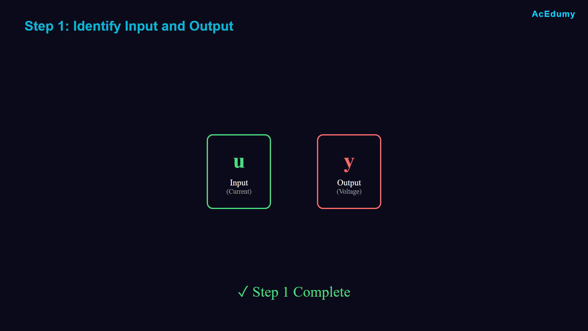
The compact integral equation is an algebraic reference with its initial-value term suppressed. Intermediate construction frames show only the blocks introduced so far. The gain frame places 1/C before integration; the narration first describes it after integration. These are equivalent for constant C and matched initial values. Equation reference cards accompany the return-path, complete, combined and comparison explanations.
Begin with input and output.
Identify the two signal roles.
Use current u as input and voltage y as output.
Keep the definitions from the RC model.
Check the current step.
Complete Step 1.
Narration transcript
Step 1 is simple. We identify input and output. Looking at our equation, u is the input and y is the output. This is exactly what we defined in lesson 4. Check. Step 1 complete.
5. Choose an integral realization
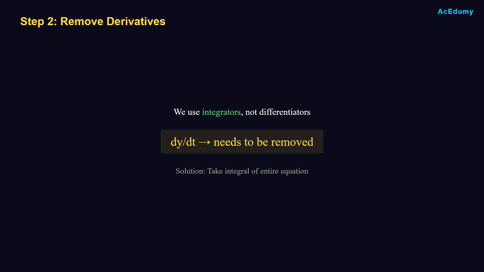
The compact integral equation is an algebraic reference with its initial-value term suppressed. Intermediate construction frames show only the blocks introduced so far. The gain frame places 1/C before integration; the narration first describes it after integration. These are equivalent for constant C and matched initial values. Equation reference cards accompany the return-path, complete, combined and comparison explanations.
Choose an integral realization.
Relate the construction to its operators.
Use integrators for this realization of the RC equation.
The model contains a first time derivative of y.
Integrate the entire equation with a common lower limit.
Narration transcript
Step 2: Remove derivatives. Why? Because in block diagrams we use integrators, not differentiators. The equation has dy dt, which is a first order derivative. To remove it, we take the integral of the entire equation.
6. Integrate both sides
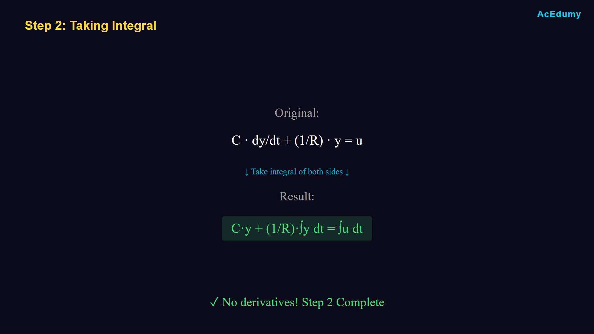
The compact integral equation is an algebraic reference with its initial-value term suppressed. Intermediate construction frames show only the blocks introduced so far. The gain frame places 1/C before integration; the narration first describes it after integration. These are equivalent for constant C and matched initial values. Equation reference cards accompany the return-path, complete, combined and comparison explanations.
Integrate the derivative term and retain its initial-value contribution.
Take the constant 1/R outside the voltage integral.
Integrate the input current over the same interval.
Compact zero-initial-value relation:
$\displaystyle C\cdot y = \int u \mathrm{d}t - \left(\frac{1}{R}\right)\cdot \int y \mathrm{d}t.$
Check the current step.
Complete Step 2 with the initial-state convention explicit.
Narration transcript
Taking the integral of both sides, integral of c dy dt becomes c times y. Integral of 1 over r times y becomes 1 over r times integral of y dt. And integral of u becomes integral of u dt. Now our equation has no derivatives. Check. Step 2: Complete.
7. Isolate the output
The compact integral equation is an algebraic reference with its initial-value term suppressed. Intermediate construction frames show only the blocks introduced so far. The gain frame places 1/C before integration; the narration first describes it after integration. These are equivalent for constant C and matched initial values. Equation reference cards accompany the return-path, complete, combined and comparison explanations.
Isolate the output y.
Put y itself alone on the left; the right side may contain its integral.
Preserve the relationships among all remaining terms.
Narration transcript
Step 3: Isolate y. We need y alone on one side, not y with an integral, not dy dt, just y by itself. The other side can have any combination of terms.
8. Rearrange the integrated equation
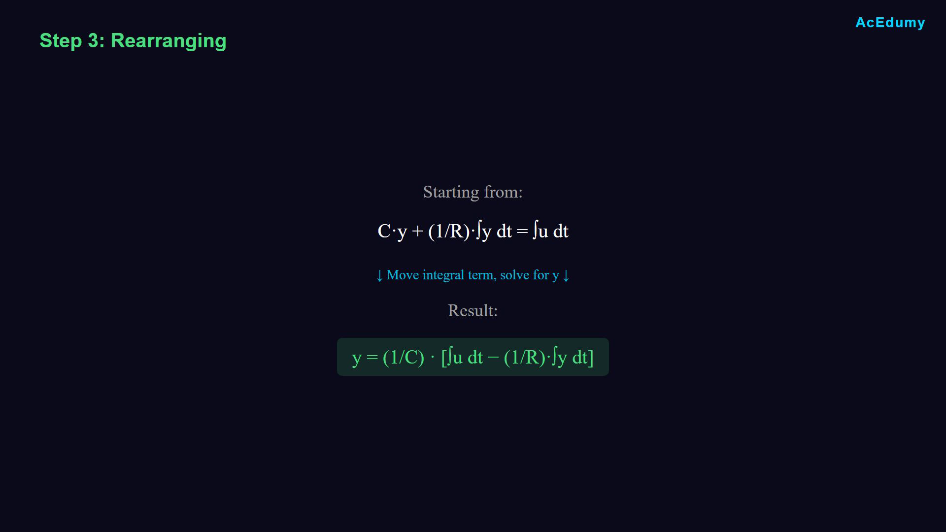
The compact integral equation is an algebraic reference with its initial-value term suppressed. Intermediate construction frames show only the blocks introduced so far. The gain frame places 1/C before integration; the narration first describes it after integration. These are equivalent for constant C and matched initial values. Equation reference cards accompany the return-path, complete, combined and comparison explanations.
Begin with the integrated RC relation.
Move the voltage-integral contribution to the right.
Compact isolated output:
$\displaystyle y = \left(\frac{1}{C}\right)\cdot \left(\int u \mathrm{d}t - \left(\frac{1}{R}\right)\cdot \int y \mathrm{d}t\right).$
Narration transcript
Starting from c times y plus 1 over r integral y dt equals integral u dt. We move the integral term to the right side. y equals 1 over c times open bracket integral u dt minus 1 over r integral y dt close bracket.
9. Combine the integrals
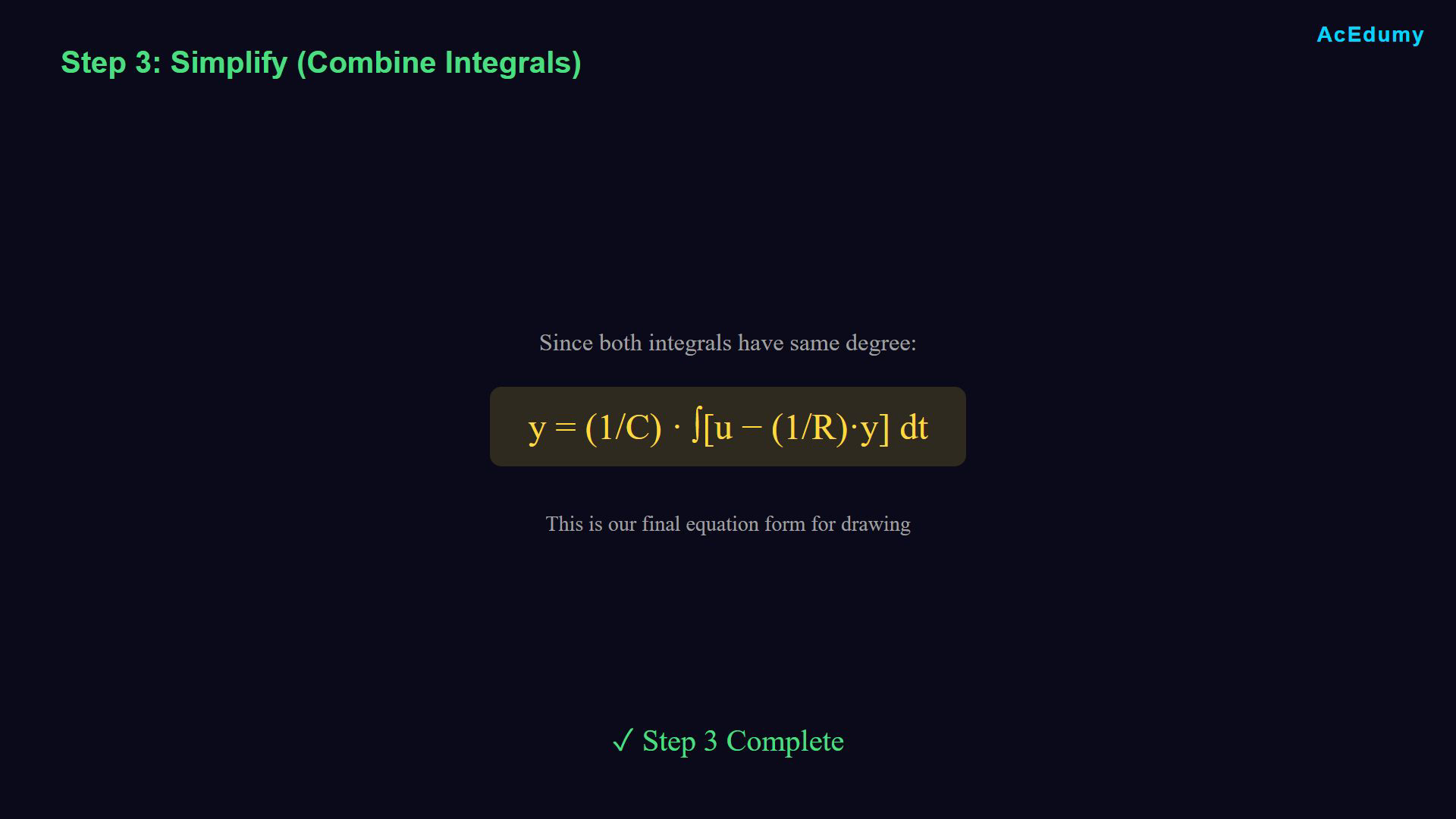
The compact integral equation is an algebraic reference with its initial-value term suppressed. Intermediate construction frames show only the blocks introduced so far. The gain frame places 1/C before integration; the narration first describes it after integration. These are equivalent for constant C and matched initial values. Equation reference cards accompany the return-path, complete, combined and comparison explanations.
Simplify using linearity of integration.
Use common integration limits and constant coefficients.
Compact combined form:
$\displaystyle y = \left(\frac{1}{C}\right)\cdot \int \left(u - \left(\frac{1}{R}\right)\cdot y\right) \mathrm{d}t.$
For a nonzero initial voltage, add the initial-value term.
Check the current step.
Complete Step 3.
Narration transcript
We can simplify this further. Since both integrals have the same degree, we combine them. y equals 1 over c times integral of open bracket u minus 1 over r times y close bracket dt. This is our final equation form. Check. Step 3: Complete.
10. Draw from inside out
The compact integral equation is an algebraic reference with its initial-value term suppressed. Intermediate construction frames show only the blocks introduced so far. The gain frame places 1/C before integration; the narration first describes it after integration. These are equivalent for constant C and matched initial values. Equation reference cards accompany the return-path, complete, combined and comparison explanations.
Draw the corresponding signal-flow blocks.
Work outward from the inner operation.
Start by placing the input and output.
Narration transcript
Step 4: Draw the block diagram. We'll build it step by step, starting from the inside and working outward. First, let's set up the input and output.
11. Place input and output
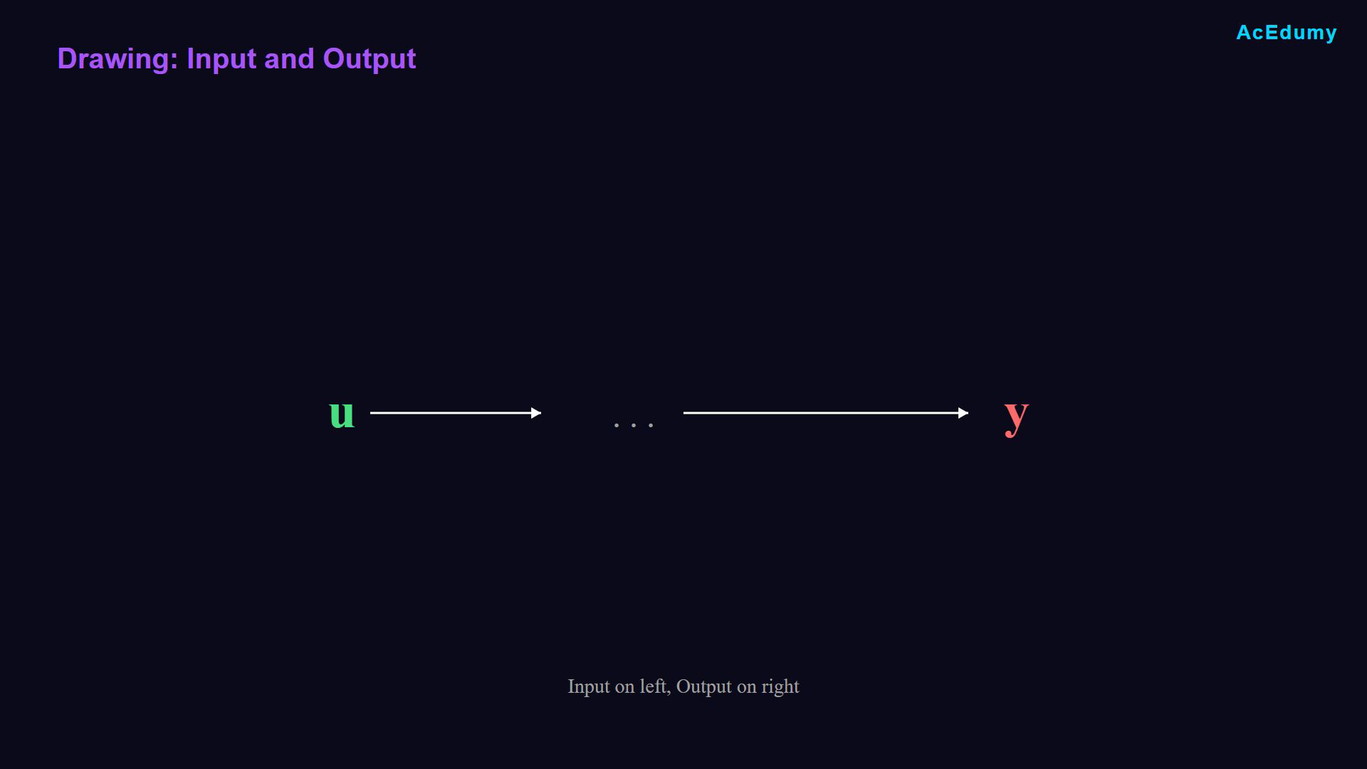
The compact integral equation is an algebraic reference with its initial-value term suppressed. Intermediate construction frames show only the blocks introduced so far. The gain frame places 1/C before integration; the narration first describes it after integration. These are equivalent for constant C and matched initial values. Equation reference cards accompany the return-path, complete, combined and comparison explanations.
Place u on the left and y on the right.
Use arrows to show signal direction.
This is a placeholder for the blocks to be added.
Narration transcript
We start by drawing input U on the left and output Y on the right. Draw an arrow from U and end with an arrow pointing to Y. We'll fill in the blocks between them.
12. Read the inner operation
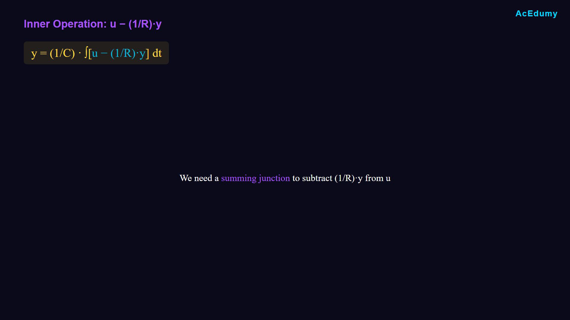
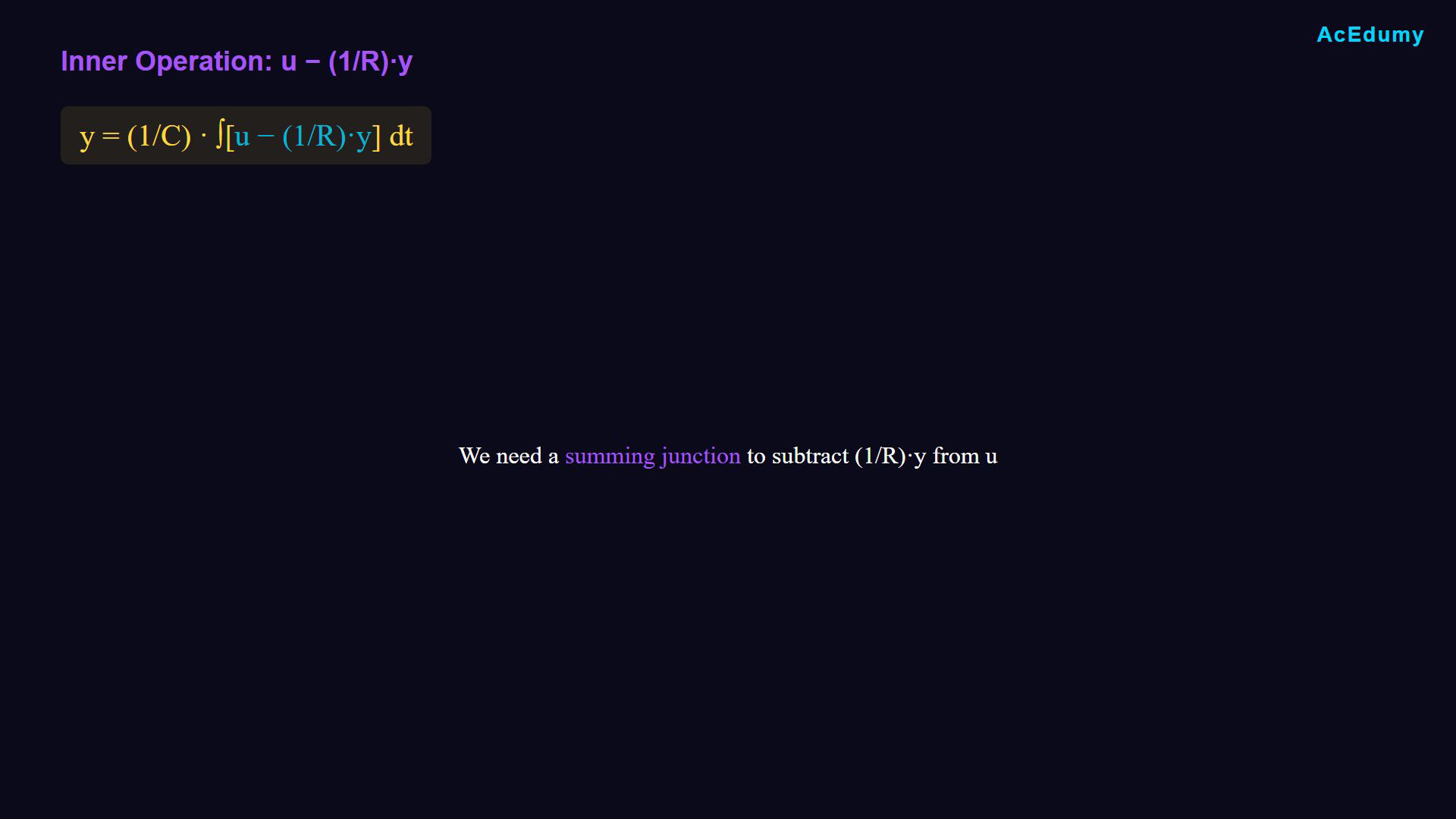
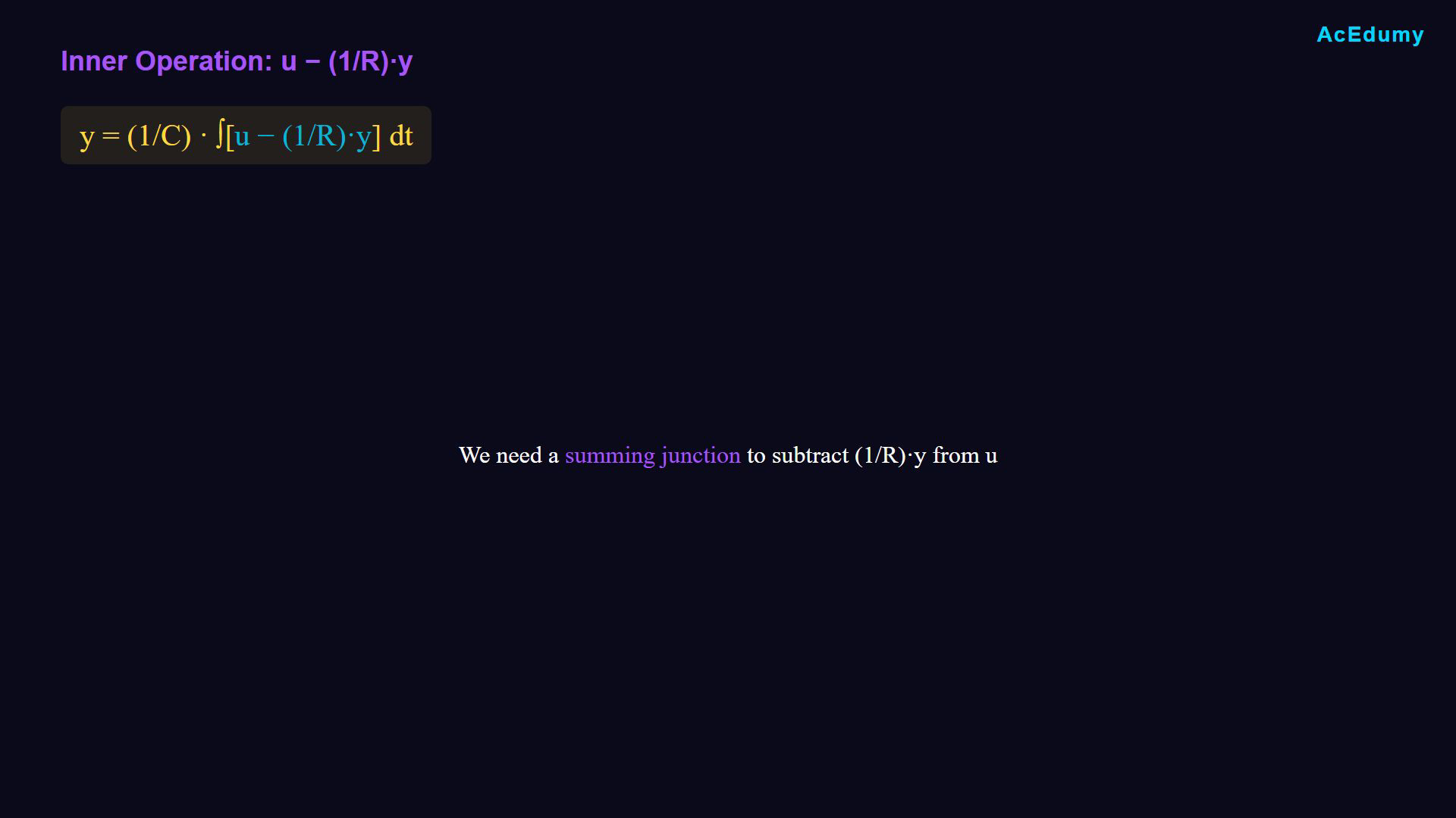
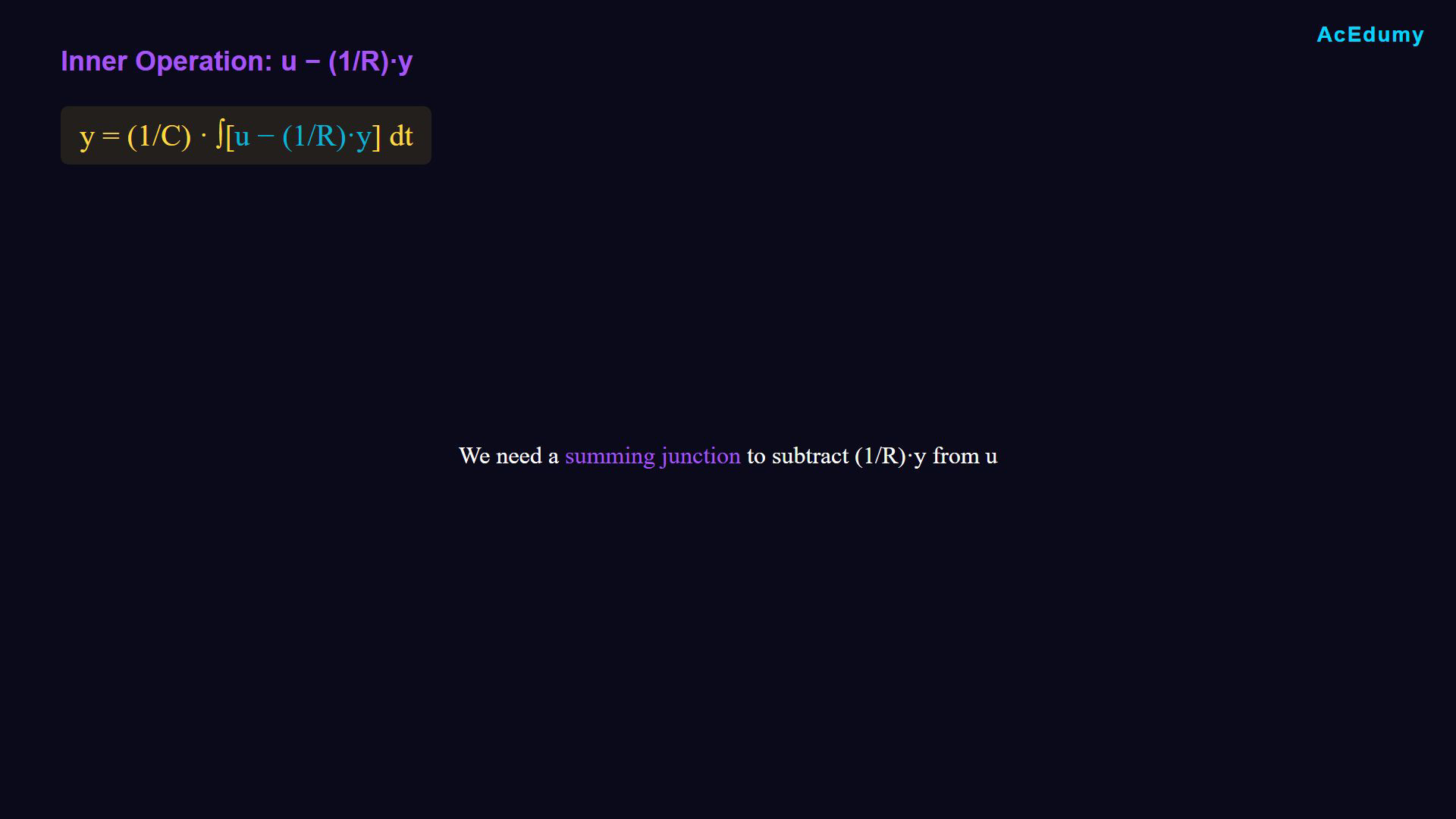
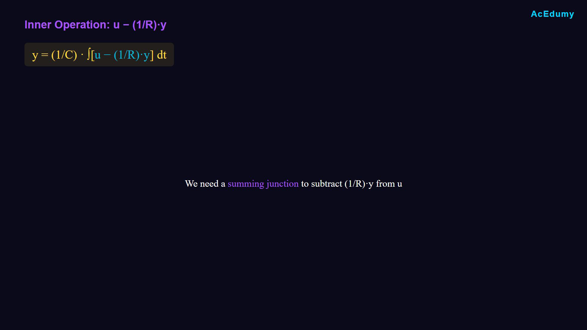
The compact integral equation is an algebraic reference with its initial-value term suppressed. Intermediate construction frames show only the blocks introduced so far. The gain frame places 1/C before integration; the narration first describes it after integration. These are equivalent for constant C and matched initial values. Equation reference cards accompany the return-path, complete, combined and comparison explanations.
Read the nested operations in the equation.
Compact output expression:
$\displaystyle y = \left(\frac{1}{C}\right)\cdot \int \left(u - \left(\frac{1}{R}\right)\cdot y\right) \mathrm{d}t.$
Inner difference:
$\displaystyle e = u - \left(\frac{1}{R}\right)\cdot y.$
Use a summing junction to form that difference.
Narration transcript
Look at the equation. y equals 1 over c integral of u minus 1 over r y dt. The innermost operation is u minus 1 over r times y. This means we need a summing junction where we subtract something from u.
13. Scale the output in the return path
The compact integral equation is an algebraic reference with its initial-value term suppressed. Intermediate construction frames show only the blocks introduced so far. The gain frame places 1/C before integration; the narration first describes it after integration. These are equivalent for constant C and matched initial values. Equation reference cards accompany the return-path, complete, combined and comparison explanations.
The returned quantity is the output scaled by 1/R.
Return-path signal:
$\displaystyle b = \left(\frac{1}{R}\right)\cdot y.$
This is an internal loop in the plant realization.
The equation reference identifies the required return gain.
Narration transcript
The term 1 over r times y comes from y itself. We need to take the output y, multiply it by 1 over r, and feed it back. This creates a feedback loop. Draw a line from y going back, add a gain block with 1 over r.
14. Assign summing-junction signs
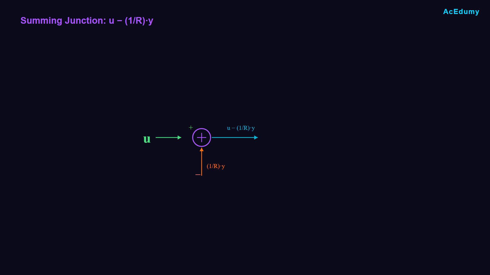
The compact integral equation is an algebraic reference with its initial-value term suppressed. Intermediate construction frames show only the blocks introduced so far. The gain frame places 1/C before integration; the narration first describes it after integration. These are equivalent for constant C and matched initial values. Equation reference cards accompany the return-path, complete, combined and comparison explanations.
Add the signed summing junction.
Connect u to its positive input.
Connect the scaled output to its negative input.
Junction output:
$\displaystyle e = u - \left(\frac{1}{R}\right)\cdot y.$
Check the complete subtracted product.
Narration transcript
Now add the summing junction. The input u enters normally with a plus sign. The feedback signal 1 over r times y enters with a minus sign. The result is u minus 1 over r times y. Exactly what we need.
15. Integrate the difference
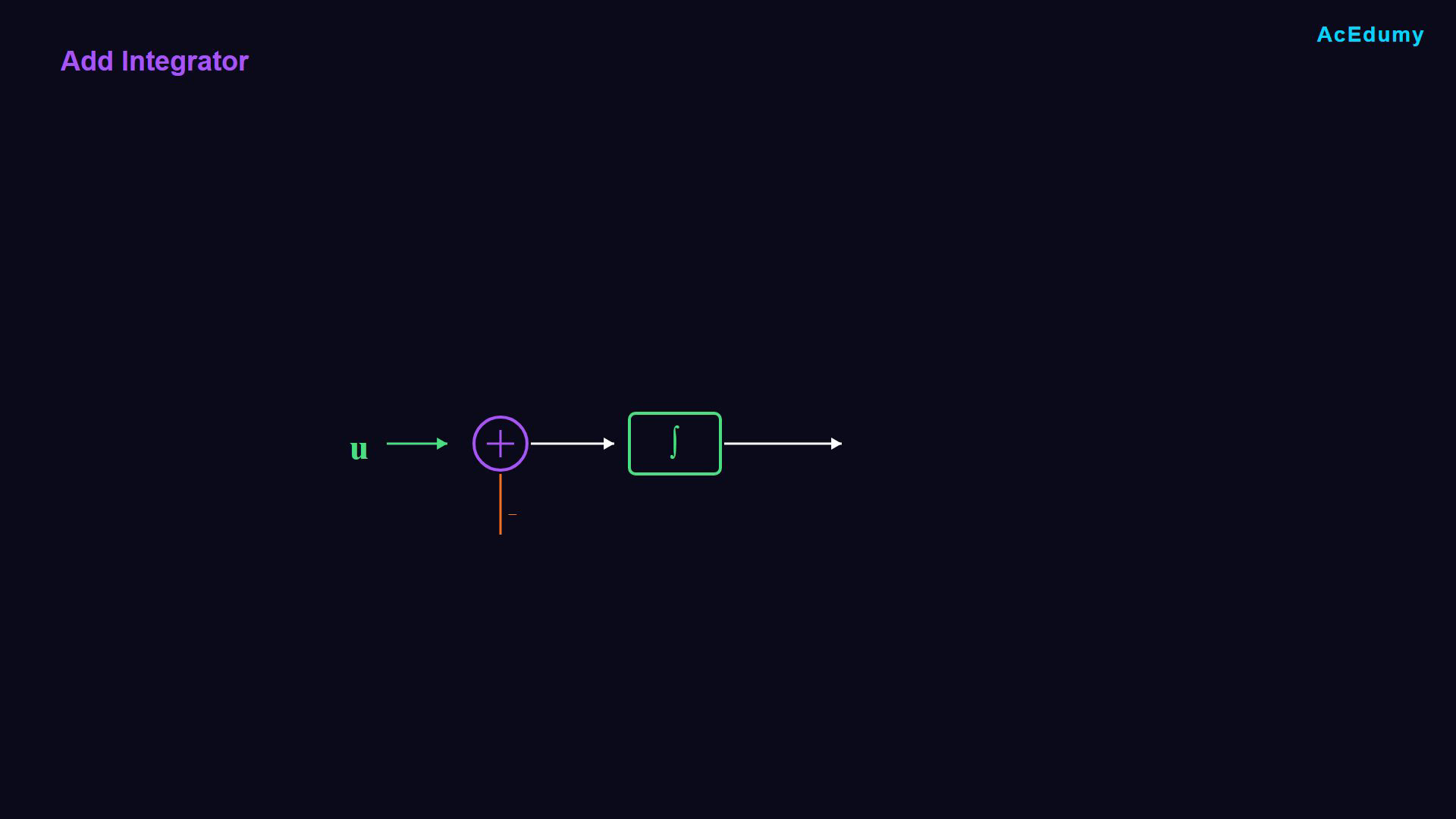
The compact integral equation is an algebraic reference with its initial-value term suppressed. Intermediate construction frames show only the blocks introduced so far. The gain frame places 1/C before integration; the narration first describes it after integration. These are equivalent for constant C and matched initial values. Equation reference cards accompany the return-path, complete, combined and comparison explanations.
Integrate the difference from the summing junction.
This frame shows an intermediate stage before the complete realization.
The integrated input is u minus the product (1/R) times y.
Narration transcript
After the summing junction, we need to integrate the result. Add an integrator block with the integral symbol. This takes u minus 1 over ry and produces the integral over time.
16. Apply the capacitance gain
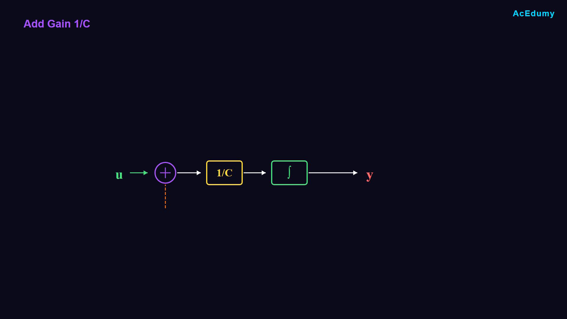
The compact integral equation is an algebraic reference with its initial-value term suppressed. Intermediate construction frames show only the blocks introduced so far. The gain frame places 1/C before integration; the narration first describes it after integration. These are equivalent for constant C and matched initial values. Equation reference cards accompany the return-path, complete, combined and comparison explanations.
Apply the constant capacitance gain.
The narration places 1/C after integration; the picture places it before.
For constant C and matched initial states, both orders yield y.
Complete the output connection and retain the return-path subtraction.
Narration transcript
Finally, we multiply by 1 over c. Add a gain block with 1 over c after the integrator. The output of this block is y. Connect it to the output arrow.
17. Read the completed realization
The compact integral equation is an algebraic reference with its initial-value term suppressed. Intermediate construction frames show only the blocks introduced so far. The gain frame places 1/C before integration; the narration first describes it after integration. These are equivalent for constant C and matched initial values. Equation reference cards accompany the return-path, complete, combined and comparison explanations.
Read the complete realization using the equation reference.
Forward rate relation:
$\displaystyle y'\left(t\right) = \left(\frac{1}{C}\right)\cdot \left(u\left(t\right) - \left(\frac{1}{R}\right)\cdot y\left(t\right)\right).$
Return y through gain 1/R to the negative summing input.
Narration transcript
Here's our complete block diagram. Input u goes to a summing junction, then through 1 over c, then through the integrator, and outputs as y. The feedback path takes y, multiplies by 1 over r, and returns to the summing junction with a minus sign.
18. Combine gain and integration
The compact integral equation is an algebraic reference with its initial-value term suppressed. Intermediate construction frames show only the blocks introduced so far. The gain frame places 1/C before integration; the narration first describes it after integration. These are equivalent for constant C and matched initial values. Equation reference cards accompany the return-path, complete, combined and comparison explanations.
Combine the constant gain and integration.
Combined operation:
$\displaystyle y = \left(\frac{1}{C}\right)\cdot \int e \mathrm{d}t.$
Match the initial output and keep the same return path.
Narration transcript
Remember from lesson 6, we can combine the gain and integrator into one block. Instead of separate 1 over c and integral blocks, we use a single block containing 1 over c times integral. Both versions give exactly the same result.
19. Compare equivalent realizations
The compact integral equation is an algebraic reference with its initial-value term suppressed. Intermediate construction frames show only the blocks introduced so far. The gain frame places 1/C before integration; the narration first describes it after integration. These are equivalent for constant C and matched initial values. Equation reference cards accompany the return-path, complete, combined and comparison explanations.
Version 1 applies gain 1/C before integration.
Version 2 combines those two operations.
Both retain the negative return path through gain 1/R.
Choose a clear drawing while preserving the complete model.
Narration transcript
Version 1 uses two blocks, gain 1 over c, followed by integrator. Version 2 uses one combined block, 1 over C integral. The feedback path with 1 over R and the summing junction remain the same. Choose whichever is clearest for your application.
20. Interpret the RC parameters
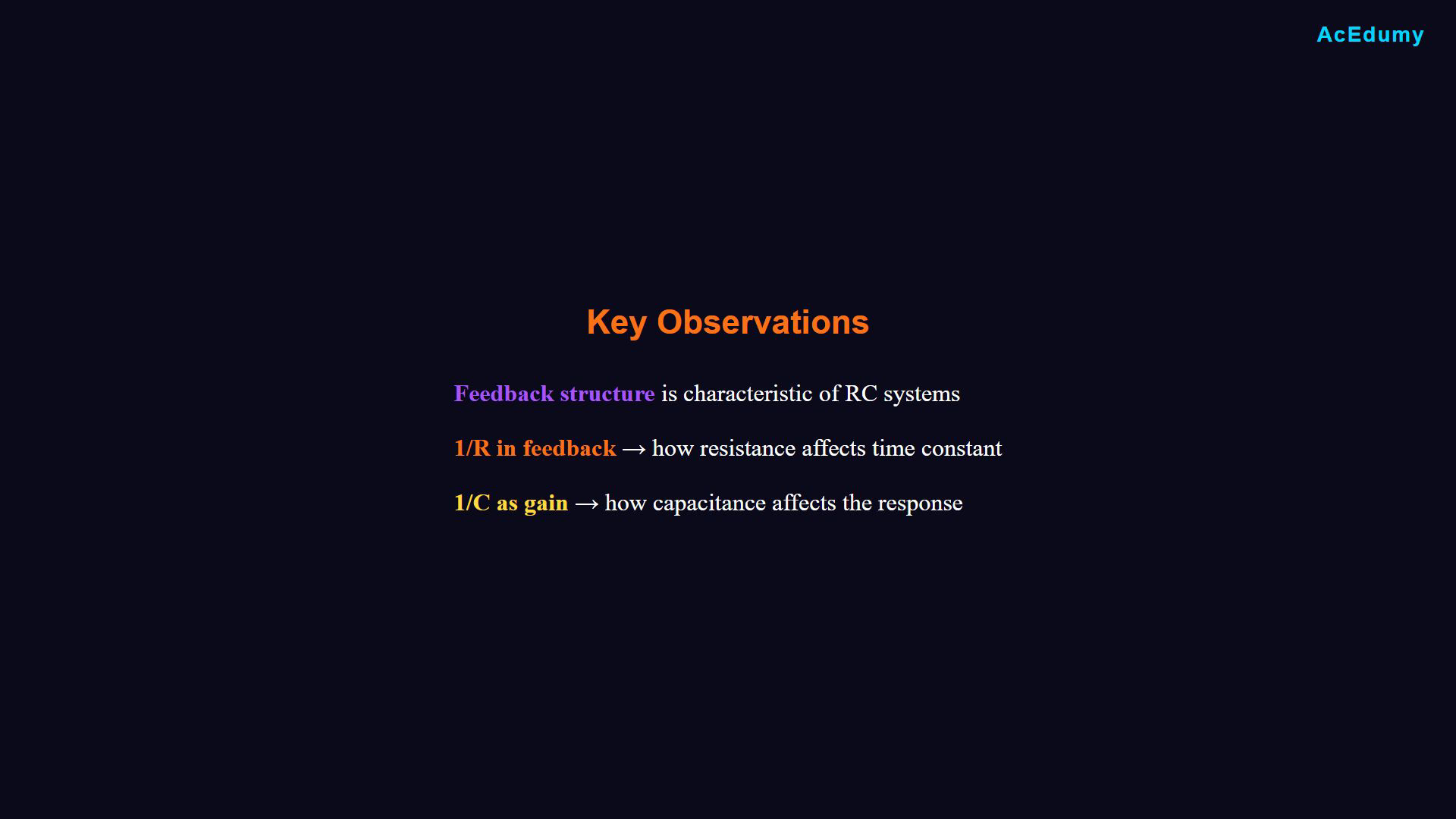
The compact integral equation is an algebraic reference with its initial-value term suppressed. Intermediate construction frames show only the blocks introduced so far. The gain frame places 1/C before integration; the narration first describes it after integration. These are equivalent for constant C and matched initial values. Equation reference cards accompany the return-path, complete, combined and comparison explanations.
Interpret the internal RC return path.
It realizes the first-order plant dynamics.
Time constant:
$\displaystyle \tau = R\cdot C.$
The internal factor 1/C affects transients; steady-state voltage/current gain is R.
Narration transcript
Notice the feedback structure. This is characteristic of first-order systems with RC dynamics. The 1 over R in feedback represents how resistance affects the time constant. The 1 over C represents how capacitance affects the gain.
21. Review the realization
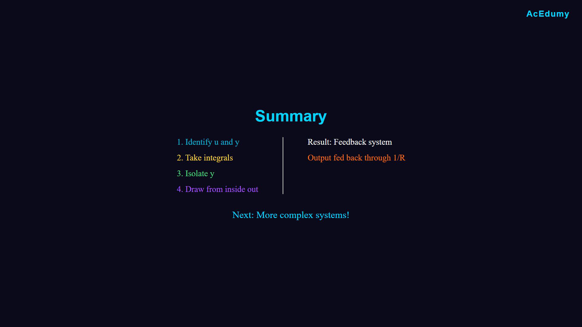
The compact integral equation is an algebraic reference with its initial-value term suppressed. Intermediate construction frames show only the blocks introduced so far. The gain frame places 1/C before integration; the narration first describes it after integration. These are equivalent for constant C and matched initial values. Equation reference cards accompany the return-path, complete, combined and comparison explanations.
Review the construction.
Convert the RC equation in four steps.
Identify current input u and voltage output y.
Integrate while retaining the initial voltage.
Isolate y.
Draw the inner operation and work outward.
The return path represents the RC plant, without a separately designed controller.
Apply the method to more complex models with all required initial states.
Continue to the next lesson.
Narration transcript
Let's summarize. We converted the RC circuit equation to a block diagram in four steps. First, identify input U and output Y. Second, take integrals to remove derivatives. Third, isolate Y on one side. Fourth, draw the diagram from inside out. The result is a feedback control system where output Y is fed back through a gain block. In the next lesson, we'll apply the same technique to more complex systems. See you then.