Control Theory · Reading a Delayed First-Order Step Response

#25 Identify gain, dead time and time constant from the final level and the onset tangent

Separate delay from lag and identify the three parameters without confusing a tangent intersection with settling.

Question

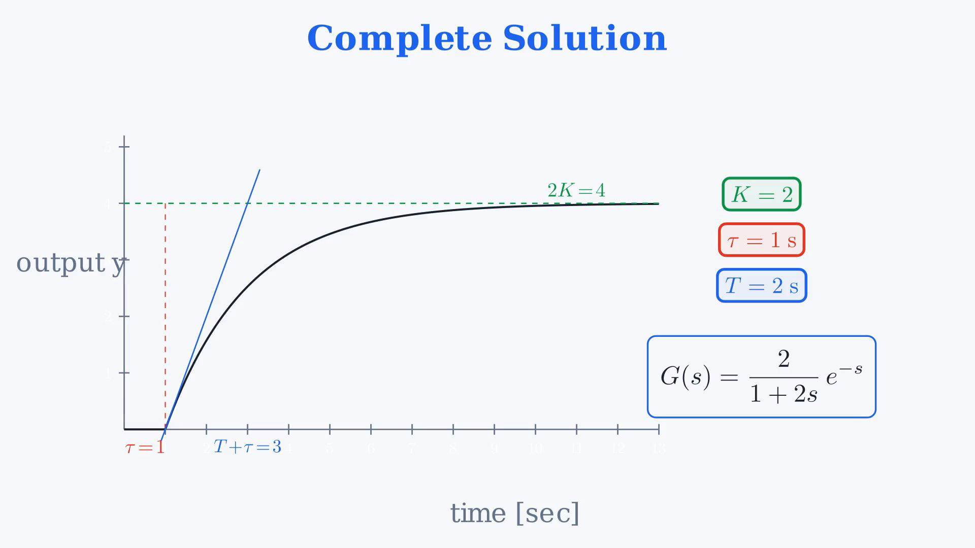
Existing final-video reference showing the delayed exponential response and its annotated results, parameter cards, tangent explanation or three-step method. — Use the numerical readings supplied in the problem and the colored result annotations. The solved graph is a qualitative reference; its pale tick labels are not needed for measurement. The straight blue tangent meets the final level at three seconds; the black response has not settled then. Read the initial slope from the right.

Assume a causal continuous-time scalar LTI plant with transfer G(s)=K exp(-tau s)/(1+T s), positive finite T, finite nonnegative delay tau, and nonzero static gain K. The example has positive gain and a positive step. There are no additional poles, zeros, direct-feedthrough terms or nonlinear effects. Begin in the zero state, with zero input/output baselines and zero prehistory, and apply the step at time zero. The source's sigma(t) denotes the Heaviside step, not an impulse or a statistical standard deviation. Its value at the single switching instant does not affect this continuous output. Use the idealized readings supplied by the example: the input step amplitude is two input units; the final output level is four output units; the output remains on the zero baseline until one second; and the tangent from the start of the rise intersects the final-output level at three seconds. These exact values are the source's mathematical worked example, not a claim of experimental measurement accuracy. The final-video solution frame visibly annotates the three values; its faint white tick labels are not the source of an additional numerical estimate. The black curve depicts the delayed exponential, the blue straight line is the onset tangent, and the green dashed line is the final-output level. Let u0 denote the nonzero step amplitude, not an initial dynamic state. In the assumed zero state, the response is zero before tau and equals K u0[1-exp(-(t-tau)/T)] for t at or after tau. Its asymptotic level y_ss is K u0. Thus K=y_ss/u0=4/2=2 output units per input unit. A static gain scales the response; it need not amplify its magnitude in every possible system. In this example it doubles it. For a biased experiment already at equilibrium, replace the absolute readings by output and input changes from their respective baselines. Arbitrary nonzero initial states require their own response and cannot be hidden by this simple ratio. The delay is measured from the known step application time to the onset of the output response. Here tau is one second. At t=tau the continuous response still equals zero and becomes positive immediately afterward; 'first leaves zero' identifies this boundary, not an attained first positive sample in a continuous-time set. If the step were applied at t0, subtract t0 from the onset time. Dead time here means no observed output change due to this input before tau. It does not prove that every internal physical variable is motionless. The bathtub and hot-tap examples are qualitative analogies, not additional governing equations. The lag time constant T determines the rate of the exponential after onset, independently of the delay. With a fixed positive final value, a smaller T gives a faster normalized rise. For t greater than tau, y'(t)=(y_ss/T) exp(-(t-tau)/T). Hence the right-hand initial slope is y_ss/T. The left slope is zero, so the ordinary two-sided derivative at the onset is not defined when y_ss is nonzero. Interpret every 'slope at tau' caption as this right-hand slope. For a positive response it is the steepest upward slope; for a negative-gain response it is the largest slope magnitude in the downward direction. The tangent is y_tan(t)=(y_ss/T)(t-tau). It reaches the final level at t_hit=tau+T. This is a geometric property of the tangent, not the actual response reaching its asymptote. Here the tangent starts at one second and crosses the level four at three seconds, so T=3-1=2 seconds. Its initial slope is two output units per second. At three seconds the actual response is only 4(1-exp(-1)), approximately 2.52848, or 63.212 percent of the final value. For the ideal exponential the exact final value is approached only as time grows without bound. A chosen two-percent settling band would first be maintained at tau+T ln(50), approximately 8.82405 seconds, not at three seconds. This optional check uses an explicitly stated tolerance. Substitute K=2, T=2 seconds and tau=1 second: G(s)=2 exp(-s)/(1+2s), where numerical times are in seconds and s has inverse-second units. The exponent is minus one second times s and is dimensionless. The lag pole is at -0.5 per second; the finite delay does not change the open plant's exponential decay rate or DC gain. The time-domain response is zero for t below one second and 4[1-exp(-(t-1)/2)] afterward. The single-state lag equation T z'+z=K u, followed by an output delay, gives the same response. Stability here concerns this given open plant; feedback stability requires a separate interconnection analysis. The three-reading method is exact for this stipulated stable first-order lag plus pure delay and ideal readings. It is not a universal identification theorem for every first-order transfer function, nor a guarantee for noisy, sampled, higher-order or nonminimum-phase responses. Check model structure, step time, baselines and input amplitude first. In measured data, an onset threshold and uncertain tangent introduce estimation error. Once those assumptions hold, identify the gain from the final change, the delay from onset, and the time constant from the tangent's horizontal interval.

Written solution and narration transcript(shows the full solution)

Below are all the lines written in the notebook together with the full narration transcript.

1. Read the measured response
Use the numerical readings supplied in the problem and the colored result annotations. The solved graph is a qualitative reference; its pale tick labels are not needed for measurement. The straight blue tangent meets the final level at three seconds; the black response has not settled then. Read the initial slope from the right.
Read the specified ideal response.
Assume a zero-state first-order lag followed by a pure delay.
Identify static gain K, positive time constant T and nonnegative delay τ.
Model family:
$\displaystyle G\left(s\right) = \left(\frac{K}{1+T\cdot s}\right)\cdot e^{-\tau \cdot s}$
Applied step:
$\displaystyle u\left(t\right) = 2\cdot \sigma \left(t\right)$
Use the supplied final level four, onset one second and tangent intersection three seconds.
Determine K, T and τ within the stipulated model family.
Narration transcript
Here is the problem. We have a system with three unknown parameters. A gain K, a first-order lag with time constant T, and a time delay tau. The transfer function is G of s equals K over one plus T s, multiplied by e to the minus tau s. We apply a step input of amplitude two, u of t equals two sigma of t. The output is recorded and shown in this graph. Our task: determine K, T, and tau from the measurement.
2. Separate gain, lag and delay
Use the numerical readings supplied in the problem and the colored result annotations. The solved graph is a qualitative reference; its pale tick labels are not needed for measurement. The straight blue tangent meets the final level at three seconds; the black response has not settled then. Read the initial slope from the right.
Separate the roles of the three parameters.
K is the static gain.
The example changes the input by two units.
Final output level:
$\displaystyle y_{\mathrm{ss}} = 2\cdot K$
The gain scales the output change; the example has positive gain.
T is the lag time constant.
It controls the exponential rise after the delay.
For fixed gain and delay, smaller positive T gives a faster normalized rise.
The bathtub is a qualitative analogy for the rate of filling.
τ is the pure output delay.
Dead time is measured from the known step application.
The output has no change due to this input before τ; internal motion is not excluded.
The hot-tap analogy illustrates a delayed observed response.
Narration transcript
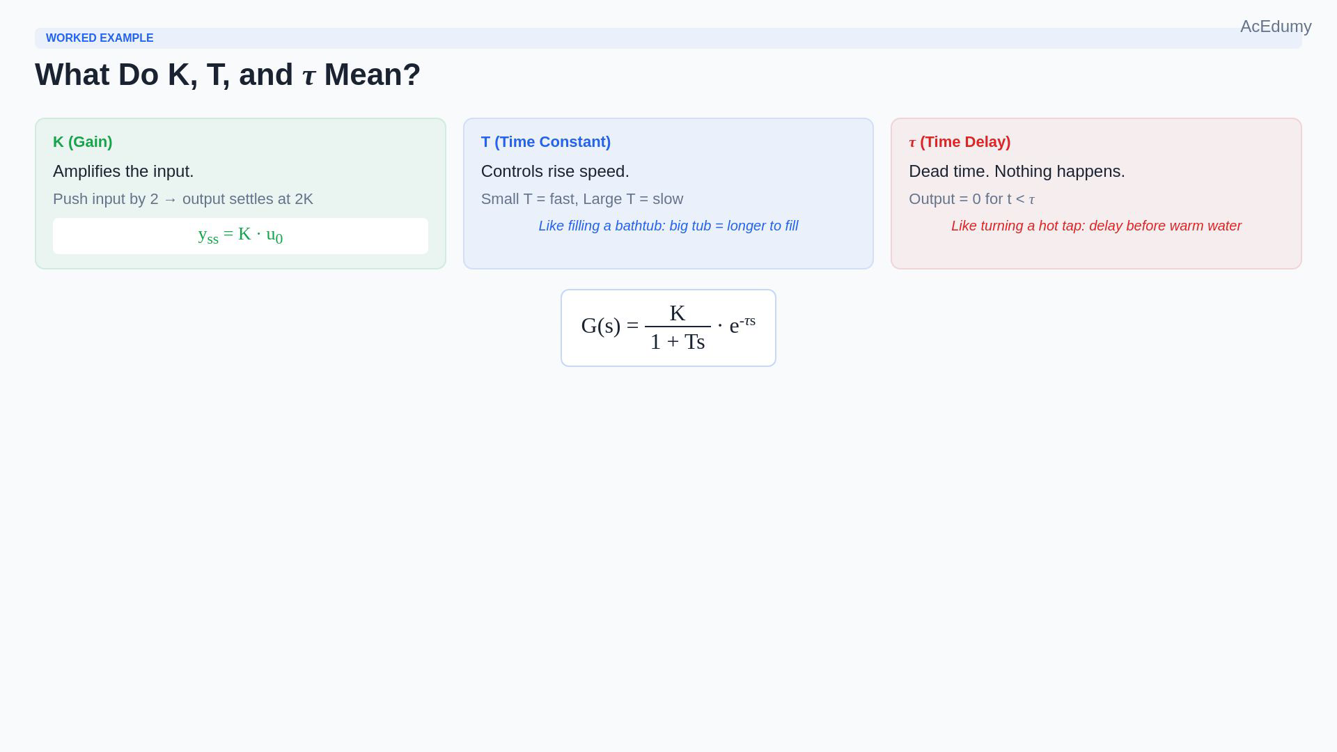
Before we read the graph, let us understand what each parameter does. K is the static gain. Imagine you push the input by two units. In steady state, the output will be two times K. So K directly tells you how much the output is amplified. T is the time constant. It controls how quickly the output rises. A small T means fast, a large T means slow. Think of it like filling a bathtub: a big bathtub takes longer to fill. And tau is the time delay. It is dead time. The system does nothing at all for tau seconds, then starts responding. Like when you turn a hot water tap: there is a delay before warm water arrives.
3. Determine the static gain
Use the numerical readings supplied in the problem and the colored result annotations. The solved graph is a qualitative reference; its pale tick labels are not needed for measurement. The straight blue tangent meets the final level at three seconds; the black response has not settled then. Read the initial slope from the right.
Find the static gain.
Use the stated final-level reading.
The exponential approaches a constant only asymptotically.
Denote that limiting level by yₛₛ.
Given final level:
$\displaystyle y_{\mathrm{ss}} = 4$
Given step amplitude:
$\displaystyle u_{0} = 2$
Zero-state static relation:
$\displaystyle y_{\mathrm{ss}} = K\cdot u_{0}$
Substitute the readings:
$\displaystyle 2\cdot K = 4$
Static gain:
$\displaystyle K =\frac{ 4}{2 }= 2$
Narration transcript
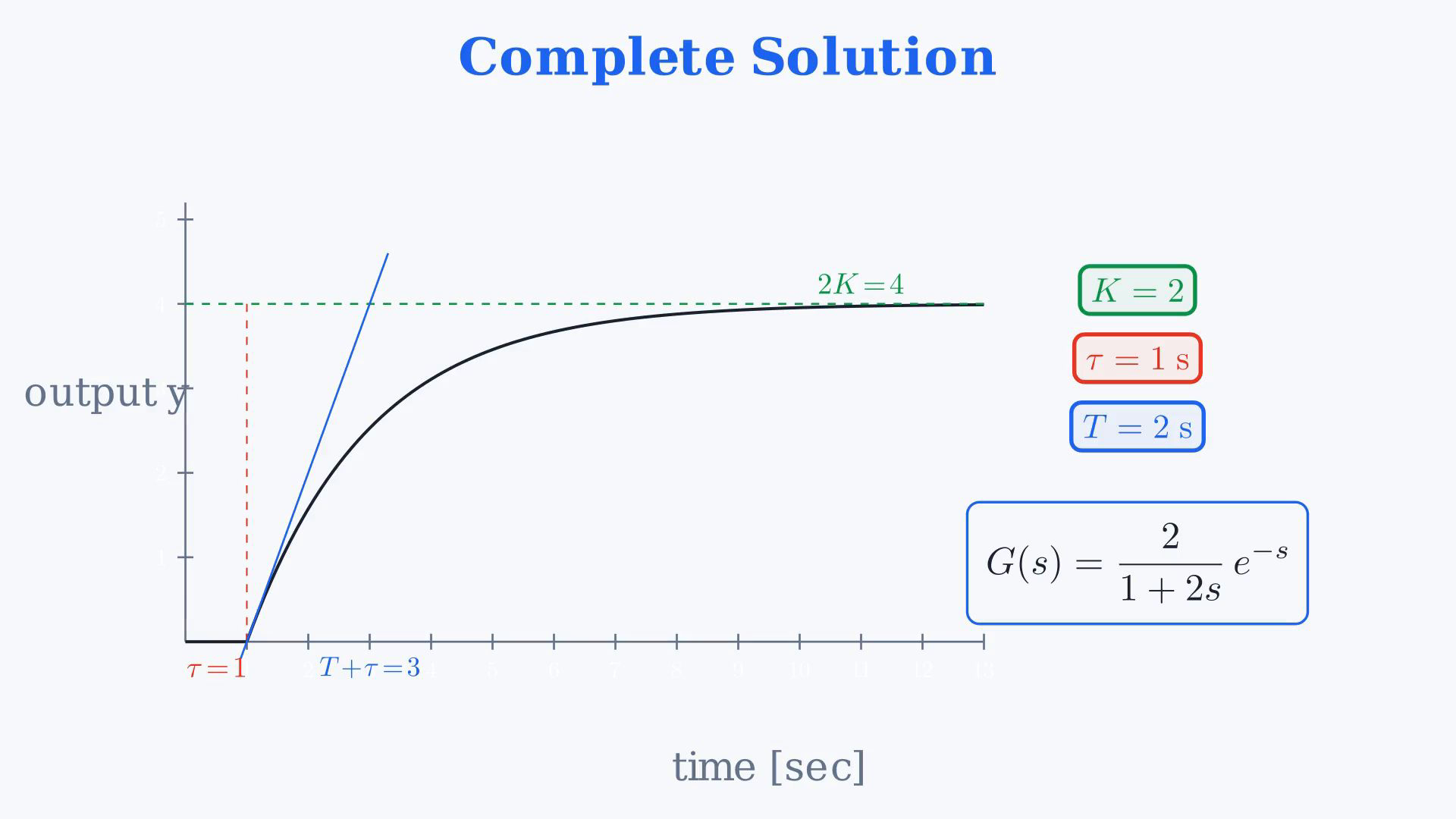
Let us start with K. Look at the graph. After a long time, the output flattens out at a constant value. This is the steady state. From the graph, the output settles at four. Now, our input was a step of amplitude two. For a first-order lag, steady state equals input times K. So two times K equals four. That gives us K equals two.
4. Locate the delay onset
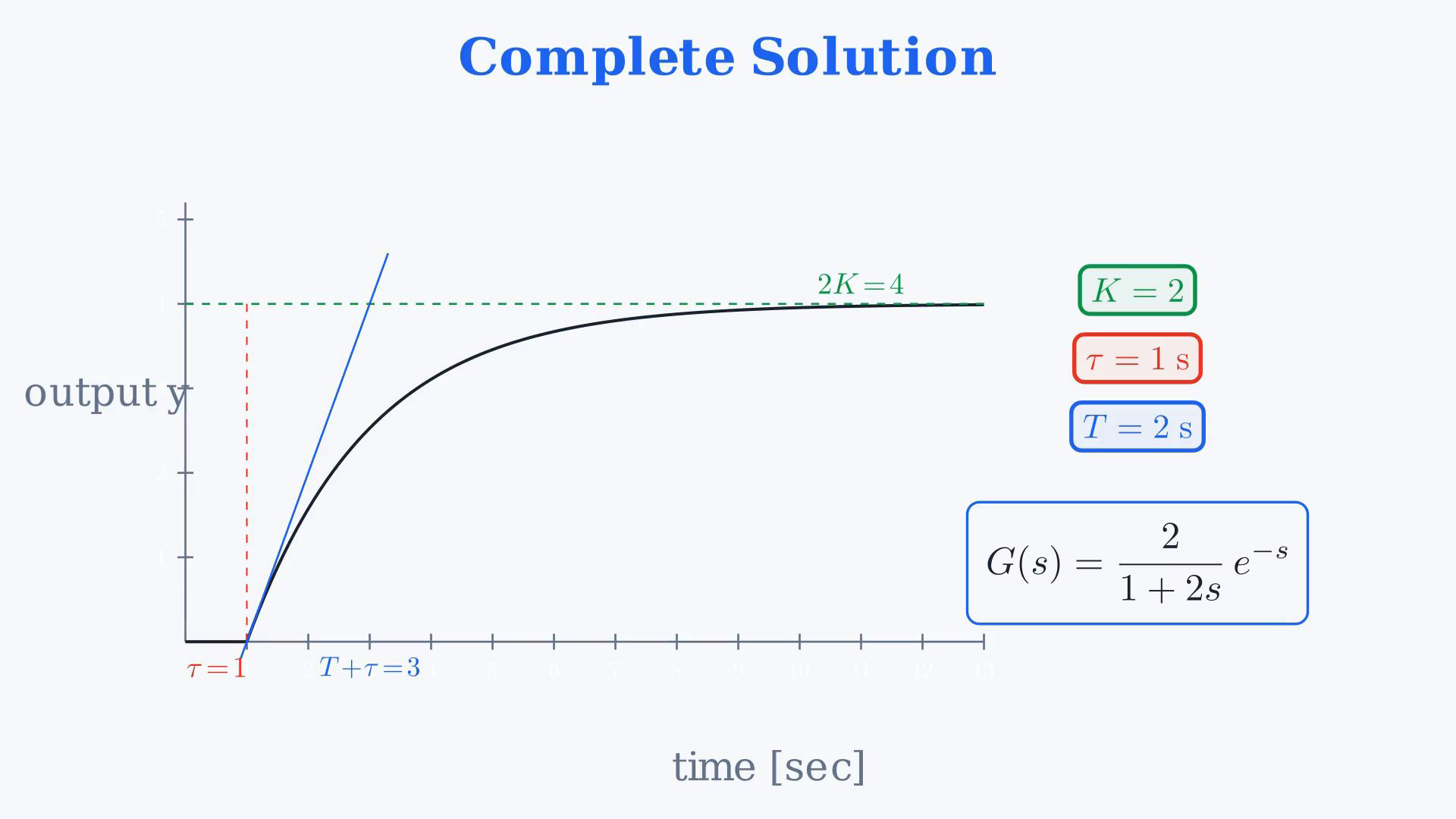
Use the numerical readings supplied in the problem and the colored result annotations. The solved graph is a qualitative reference; its pale tick labels are not needed for measurement. The straight blue tangent meets the final level at three seconds; the black response has not settled then. Read the initial slope from the right.
Locate the output delay.
Start at the known input-step time.
The output stays on its zero baseline before onset.
No output change is observed in that interval.
That flat interval is the dead time for this ideal response.
This describes the output response to the step.
The supplied onset time is one second after the input step.
At the onset the output is still zero, then rises immediately afterward.
Delay in seconds:
$\displaystyle \tau = 1$
Narration transcript
Next, the time delay tau. Look at the very beginning of the graph. The output stays exactly at zero. It does not move at all. This flat region is the delay. The system has not started responding yet. From the graph, this zero region lasts until time equals one second. At that moment, the curve starts rising. So tau equals one second.
5. Use the right-hand initial tangent
Use the numerical readings supplied in the problem and the colored result annotations. The solved graph is a qualitative reference; its pale tick labels are not needed for measurement. The straight blue tangent meets the final level at three seconds; the black response has not settled then. Read the initial slope from the right.
Find the lag time constant separately from the delay.
Use the tangent on the rising side of the onset.
Explain the tangent construction.
For t after τ:
$\displaystyle y\left(t\right) = y_{\mathrm{ss}}\cdot \left(1-e^{-(t-\tau )/T}\right)$
For this positive response, the right-hand initial slope is the steepest upward slope.
Extend that initial tangent as a straight line.
Right-hand initial slope:
$\displaystyle b =\frac{ y_{\mathrm{ss}}}{T}$
Tangent line:
$\displaystyle y_{\mathrm{tan}}\left(t\right) = \left(\frac{y_{\mathrm{ss}}}{T}\right)\cdot \left(t-\tau \right)$
Tangent intersection time:
$\displaystyle t_{\mathrm{hit}} = \tau +T$
Narration transcript
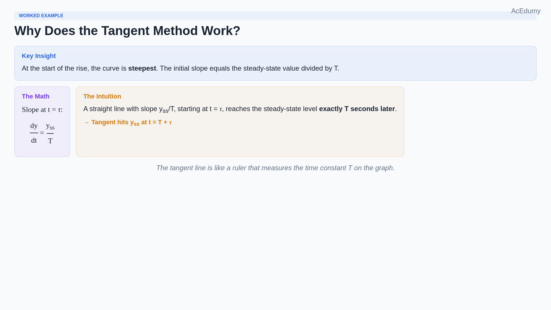
Now we need to find T. We will use the tangent line method. But first, why does this work? For a first-order lag, the step response rises following an exponential curve. At the very beginning of the rise, the curve is steepest. If you draw a straight line along that steepest slope, it acts like a ruler measuring the time constant. Mathematically, the initial slope equals the steady state value divided by T. So a straight line with that slope, starting from tau, will reach the steady state level exactly T seconds later. That is why the tangent line meets the steady state at time T plus tau.
6. Measure the time constant
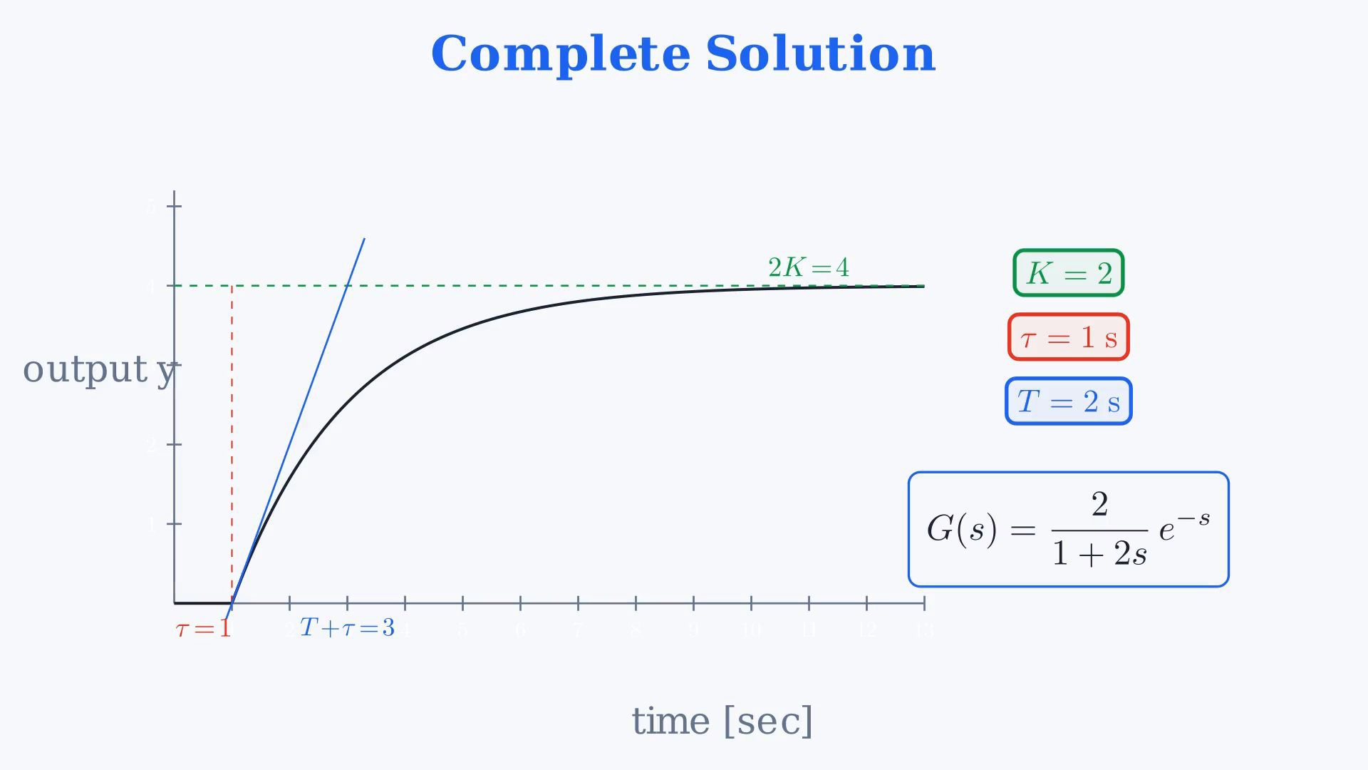
Use the numerical readings supplied in the problem and the colored result annotations. The solved graph is a qualitative reference; its pale tick labels are not needed for measurement. The straight blue tangent meets the final level at three seconds; the black response has not settled then. Read the initial slope from the right.
Apply the tangent construction to the given readings.
The rising side begins at one second.
Draw the tangent using the right-hand slope at onset.
The tangent meets the level four at three seconds; the actual response remains below it.
Intersection time in seconds:
$\displaystyle T+\tau = 3$
Known delay in seconds:
$\displaystyle \tau = 1$
Time constant in seconds:
$\displaystyle T = 3-1 = 2$
Narration transcript
Let us apply this. At time equals tau, which is one second, the response starts rising. We draw a tangent line at that point. Following this tangent line upward, it hits the steady state value of four at time equals three seconds. So T plus tau equals three. We already know tau is one. Therefore T equals three minus one equals two seconds.
7. Write the identified transfer
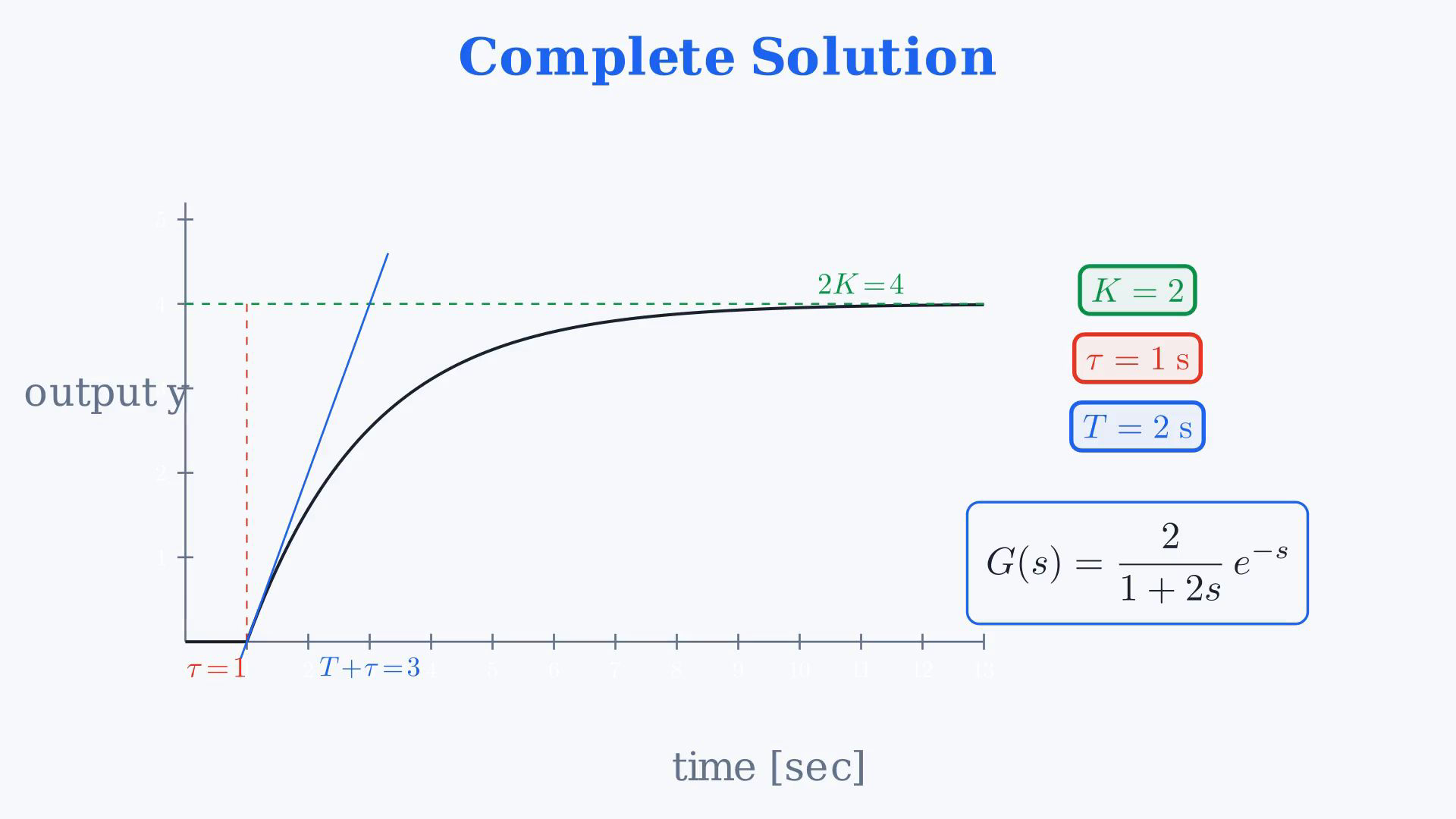
Use the numerical readings supplied in the problem and the colored result annotations. The solved graph is a qualitative reference; its pale tick labels are not needed for measurement. The straight blue tangent meets the final level at three seconds; the black response has not settled then. Read the initial slope from the right.
Collect the three identified parameters.
The result is gain two, delay one second and lag time constant two seconds.
Identified transfer:
$\displaystyle G\left(s\right) = \left(\frac{2}{1+2\cdot s}\right)\cdot e^{-s}$
This is the stipulated stable first-order lag with a one-second output delay.
Narration transcript
Now we have all three parameters. K equals two, tau equals one second, and T equals two seconds. Plugging these into the transfer function: G of s equals two over one plus two s, times e to the minus s. This is a first-order lag with gain two, time constant two seconds, and a one second delay.
8. Review the identification assumptions
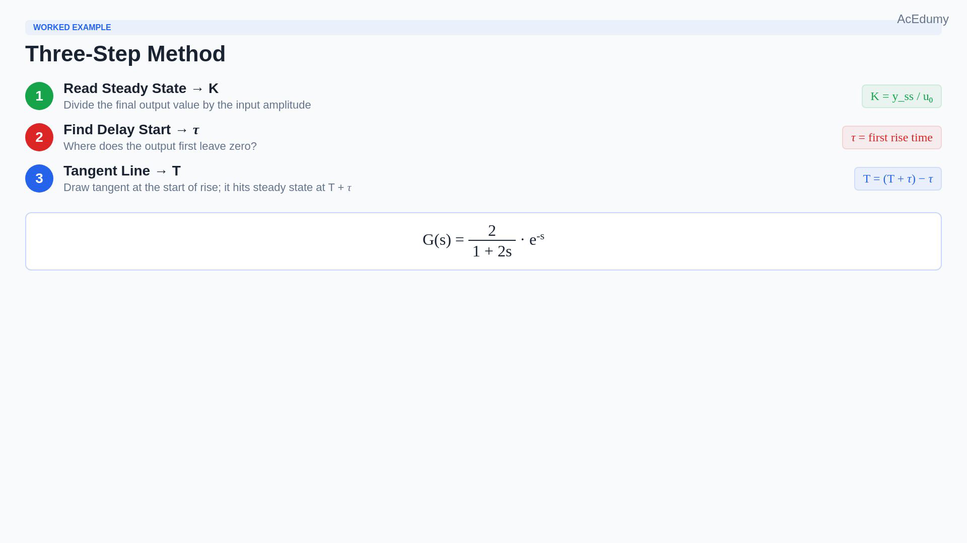
Use the numerical readings supplied in the problem and the colored result annotations. The solved graph is a qualitative reference; its pale tick labels are not needed for measurement. The straight blue tangent meets the final level at three seconds; the black response has not settled then. Read the initial slope from the right.
Review the method for the assumed zero-state lag-plus-delay family.
Divide the final output change by the nonzero input-step change.
Gain from the readings:
$\displaystyle K =\frac{ y_{\mathrm{ss}}}{u_{0}}$
Locate the onset relative to the known step application time.
That elapsed time gives the delay τ.
Use the tangent from the rising side of the onset.
Its intersection with the final level gives the time τ plus T.
Time constant:
$\displaystyle T = t_{\mathrm{hit}}-\tau$
These readings identify this model when its structure and measurement assumptions hold.
Narration transcript
Let us review the three-step method for reading any first-order step response. Step one: read the steady state value and divide by the input amplitude. That gives K. Step two: find where the output first leaves zero. That time is the delay tau. Step three: draw a tangent at the start of the rise. Where it hits the steady state gives T plus tau. Subtract tau to get T. Three simple readings, and you have the complete transfer function.