Control Theory · Root Locus, Strict Stability and Stable Oscillation
#43 Separate the origin crossing, real-pole breakaway and infinite-gain limits
Use one quadratic characteristic polynomial to identify a strict stability interval, the stable complex-pole interval and the nonnegative-gain root locus.
Question
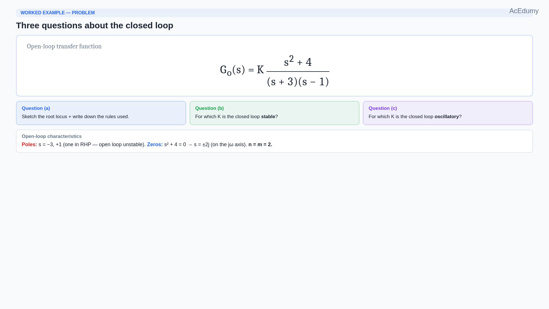
Consider unity negative feedback with open-loop transfer function G_o(s)=K(s²+4)/[(s+3)(s-1)]. The negative-feedback sign is specified by the solution equation1+G_o=0. K is a real gain; the root-locus sketch uses nonnegative K. Find the closed-loop characteristic equation, strict stability range, and stable oscillatory range, and sketch the nonnegative-gain locus with its rules. The solution explicitly intersects complex poles with stability for part(c). Do not call the negative-gain unstable complex-pole branch stable oscillation. No particular initial state, physical units, or input waveform is given. Oscillatory refers to nonreal natural modes, not a claim that every specially chosen input or initial condition excites them. Write D(s)=(s+3)(s-1)=s²+2s-3 and N(s)=s²+4. The characteristic polynomial is P_K=D+K*N=(1+K)s²+2s+4K-3. The closed-loop reference map is T=K*N/P_K. Because the open loop is biproper, the feedback algebraic loop requires1+K nonzero; K=-1 is excluded as singular, and the nonnegative-gain sketch is well posed. A reduced linear polynomial obtained formally at K=-1 does not restore that well-posed feedback. For nonzero K, neither numerator zero cancels a characteristic root: P_K(2j)=-7+4j and P_K(-2j)=-7-4j. At zero gain the minimal reference map is zero, but the disconnected plant still has its unstable+1 internal mode; the root-locus starting poles mean roots of P_0 or limits from positive gain, not poles of the identically zero reference map. The real quadratic coefficients are a=1+K,b=2,c=4K-3. Since b is fixed positive, its two roots are strictly in the left half plane if and only if a and c are positive: K>-1 and K>3/4, whose intersection is K>3/4. More generally a real quadratic requires all coefficients of the same nonzero sign after normalization; multiplying a stable polynomial by minus one cannot change its roots. The all-positive wording is used here with b=2. At K=3/4, P=(7/4)s²+2s has simple roots0 and-8/7. This is not asymptotic or BIBO stability. Its zero-state unit-step output is unbounded because T/s has a double pole at the origin. The zero eigenvalue can give bounded homogeneous motion, so avoid using marginally unstable as a universal Lyapunov classification. The source's boundary label and strict inequality settle the requested convention. For nonnegative K below3/4, the product of the two roots is negative, giving one positive and one negative root. For oscillatory natural modes require discriminant Δ=b²-4ac<0. Here Δ=4-4(1+K)(4K-3)=16-16K²-4K=-4(4K²+K-4). The boundary gains are K_plus=(sqrt(65)-1)/8 and K_minus=(-1-sqrt(65))/8. They are approximately0.8827822185 and-1.1327822185. Complex poles occur for K<K_minus or K>K_plus. The negative branch has positive real parts and is unstable. The stable oscillatory answer is K>K_b, where K_b=K_plus. Decimal0.883 is an approximation to the boundary, not an exact substitute in an inequality near it. For3/4<K<K_b there are two distinct negative real poles. At K=K_b there is one repeated negative real pole s_b=-1/(1+K_b)=(7-sqrt(65))/2, approximately-0.5311288741. A repeated real pole can produce t times an exponential but has no nonzero-frequency sinusoidal mode. Only strictly above K_b does the conjugate pair appear. Thus the casual phrase moment oscillation begins denotes this boundary, consistently with the displayed strict inequality. For K>K_b, the poles are -1/(1+K) plus or minus j*sqrt(4K²+K-4)/(1+K). Their real parts are negative for every finite such gain; as K tends to positive infinity the real parts tend to zero from below and imaginary parts tend to plus or minus2. No finite gain places a pole at either open-loop imaginary zero. Larger K in this interval does not mean a faster exponential decay: its real parts approach zero. The final gain-ten plot's deep-complex wording describes a larger imaginary part, not deeper placement in the left half plane. The gain-two real part is-1/3 and gain-ten real part-1/11. Zeros, residues and input/initial conditions also matter for full transient shape; poles alone determine modal rates and frequencies. For the nonnegative-gain locus, there are two branches starting at plant poles-3 and+1 and approaching zeros+2j and-2j. Pole and zero counts n=m=2 give no asymptotes. On the real line away from singular endpoints, the odd-count rule uses real open-loop poles and zeros to the right. Only the interval(-3,1) has an odd count; include endpoints as K=0 limits. Equivalently solving P_K(s)=0 for real s gives K(s)=-(s²+2s-3)/(s²+4), which is nonnegative exactly on[-3,1]. Its derivative is2(s²-7s-4)/(s²+4)². The stationary point(7-sqrt(65))/2 lies on this interval and gives K_b. The other stationary point(7+sqrt(65))/2 lies off the positive-gain locus and belongs to the negative-gain branch; do not add it to this sketch. Substitute s=j*omega into P_K. The real equation is -(1+K)*omega²+4K-3=0, with the minus sign applying to the whole coefficient1+K. The imaginary equation is2omega=0, so omega=0 and K=3/4. This is the sole imaginary-axis crossing for finite real gain; the infinite-gain limiting zeros are separate. At K=3/4 the right branch crosses the origin; immediately above it both roots are negative. They meet at s_b and K_b, then leave the real line as a conjugate pair. For a complex pole x+jy, the sum and product identities give x=-1/(1+K) and x²+y²=4+7x. Equivalently the complex arcs lie on (x-7/2)²+y²=65/4, restricted to the left arc from x=s_b to x approaching0 from below. This independently checks the qualitative sketch. At K=0.5 one pole is positive; at K=0.8 both are negative real; at K=2 and10 they are stable conjugate pairs. Use exact boundaries when deciding these regions.
Written solution and narration transcript(shows the full solution)
Below are all the lines written in the notebook together with the full narration transcript.
1. Read the unity-feedback problem
The gain three quarters is a stability boundary, and the positive discriminant boundary has a repeated real pole. Strict inequalities exclude both endpoints from their respective open intervals. Imaginary zeros are approached only as gain tends to infinity. The final example with gain ten has larger imaginary parts but real parts closer to zero than the gain-two example. The problem.Open-loop transfer function:K is a free gain.Use unity negative feedback, as specified by the characteristic equation in the solution.Question a — sketch the root locus, and write down the rules used.Question b — for which values of K is the closed loop stable?Part c: find the stable oscillatory range, as obtained by intersecting complex poles with the stability condition.Notice the open-loop characteristics already make this interesting.Open-loop poles:The pole at plus one is in the right half plane — the open loop is unstable.We want feedback to fix that.Open-loop zero equation:Open-loop zeros:Pure imaginary zeros, sitting on the j omega axis.Pole and zero counts:Narration transcript
The problem. We are given the open-loop transfer function G sub o of s equals K times s squared plus four, divided by s plus three times s minus one. K is a free gain. The system is in a unity feedback loop, so we ask three questions about the closed loop. Question a — sketch the root locus, and write down the rules used. Question b — for which values of K is the closed loop stable? Question c — for which values of K is the closed loop oscillatory? Notice the open-loop characteristics already make this interesting. Open-loop poles — minus three, and plus one. The pole at plus one is in the right half plane — the open loop is unstable. We want feedback to fix that. Open-loop zeros — solve s squared plus four equals zero. s equals plus or minus two j. Pure imaginary zeros, sitting on the j omega axis. Two open-loop poles, two open-loop zeros — n equals m equals two.
2. Use one characteristic equation

The gain three quarters is a stability boundary, and the positive discriminant boundary has a repeated real pole. Strict inequalities exclude both endpoints from their respective open intervals. Imaginary zeros are approached only as gain tends to infinity. The final example with gain ten has larger imaginary parts but real parts closer to zero than the gain-two example. The strategy.Three questions, but they all live on the same closed-loop characteristic equation.Build it once, then read three different facts off of it.Step one — write the closed-loop characteristic equation.Characteristic equation before expansion:The result is a quadratic in s with K-dependent coefficients.Step two — stability.The CE is second order.For this quadratic with a positive linear coefficient, strict stability requires all three coefficients to be positive.Get a K range.Step three — oscillation.Nonreal conjugate poles produce oscillatory natural modes; within the stable range these modes decay.Compute the discriminant and find where it goes negative.Step four — root locus.Use the standard rules — real-axis segments, asymptotes, j omega axis crossing — to sketch the path of the closed-loop poles as K varies from zero to infinity.Three questions, one characteristic polynomial, four short calculations.Let us begin.Narration transcript
The strategy. Three questions, but they all live on the same closed-loop characteristic equation. Build it once, then read three different facts off of it. Step one — write the closed-loop characteristic equation. One plus G sub o of s equals zero, expanded. The result is a quadratic in s with K-dependent coefficients. Step two — stability. The CE is second order. Apply the necessary condition for a quadratic — every coefficient strictly positive. Get a K range. Step three — oscillation. A second-order system oscillates when its roots are complex — which happens when the discriminant is negative. Compute the discriminant and find where it goes negative. Step four — root locus. Use the standard rules — real-axis segments, asymptotes, j omega axis crossing — to sketch the path of the closed-loop poles as K varies from zero to infinity. Three questions, one characteristic polynomial, four short calculations. Let us begin.
3. Expand and collect the quadratic
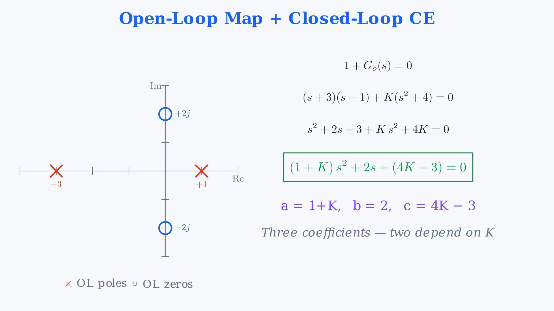
The gain three quarters is a stability boundary, and the positive discriminant boundary has a repeated real pole. Strict inequalities exclude both endpoints from their respective open intervals. Imaginary zeros are approached only as gain tends to infinity. The final example with gain ten has larger imaginary parts but real parts closer to zero than the gain-two example. Step one — closed-loop characteristic equation.Set the feedback characteristic equation:Substitute the complete numerator and denominator:Multiply through by the denominator.Polynomial equation after clearing the denominator:Expand the first product.Expand the plant denominator:Add the K-weighted zero polynomial.Gain-weighted numerator:Collect by power of s.Quadratic coefficient:Linear coefficient:Constant coefficient:Closed-loop characteristic equation:Three coefficients, two of them carry K.This single quadratic is the key — we will mine three different facts from it.Narration transcript
Step one — closed-loop characteristic equation. Set one plus G sub o of s equal to zero. One plus K times s squared plus four, all over s plus three times s minus one, equals zero. Multiply through by the denominator. s plus three times s minus one, plus K times s squared plus four, equals zero. Expand the first product. s plus three times s minus one is s squared minus s plus three s minus three, which simplifies to s squared plus two s minus three. Add the K-weighted zero polynomial. K s squared plus four K. Collect by power of s. Coefficient of s squared — one plus K. Coefficient of s — two. Constant — minus three plus four K, or four K minus three. The closed-loop characteristic equation is one plus K, times s squared, plus two s, plus four K minus three, equals zero. Three coefficients, two of them carry K. This single quadratic is the key — we will mine three different facts from it.
4. Find the strict stability interval
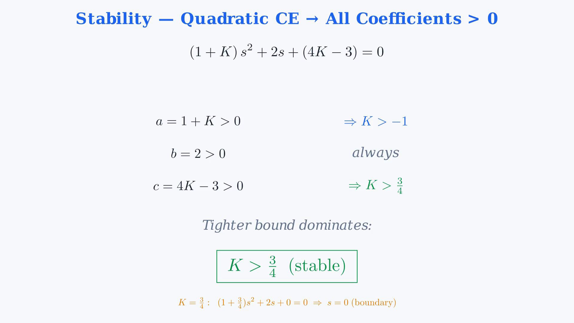
The gain three quarters is a stability boundary, and the positive discriminant boundary has a repeated real pole. Strict inequalities exclude both endpoints from their respective open intervals. Imaginary zeros are approached only as gain tends to infinity. The final example with gain ten has larger imaginary parts but real parts closer to zero than the gain-two example. Step two — stability.Quadratic and its coefficients:Since the linear coefficient is positive, this real quadratic has strictly left-half-plane roots exactly when all three coefficients are positive.For a real quadratic with positive leading coefficient, the positive-coefficient condition is necessary and sufficient for strict stability.Walk through the three coefficients.Leading coefficient:Linear coefficient:No constraint on K.Constant coefficient:Combine.The leading-coefficient inequality requires gain greater than minus one.The constant-coefficient inequality requires gain greater than three quarters.Three quarters is the tighter bound, so it dominates.Stability range.Strict stability requires gain greater than three quarters.At gain three quarters, one root is at the origin: this is the boundary and is not strictly stable or BIBO stable.Below three quarters the well-posed closed loop fails strict stability.Part b: the closed loop is strictly stable exactly for gain greater than three quarters.Narration transcript
Step two — stability. The characteristic equation is a quadratic — a s squared plus b s plus c equals zero, with a equals one plus K, b equals two, and c equals four K minus three. For a quadratic, stability has a clean shortcut — the system is stable if and only if every coefficient is strictly positive. This is the Routh-Hurwitz necessary condition, which is also sufficient at order two. Walk through the three coefficients. a positive — one plus K greater than zero — gives K greater than minus one. b positive — two greater than zero — always true. No constraint on K. c positive — four K minus three greater than zero — gives K greater than three quarters. Combine. The first inequality demands K greater than minus one. The third demands K greater than three quarters. Three quarters is the tighter bound, so it dominates. Stability range. K must be strictly greater than three quarters. At K equals three quarters exactly, the constant term vanishes — one root sits at the origin, marginally unstable. Below three quarters, stability is lost. Answer to question b — closed loop is stable for K greater than three quarters.
5. Find the stable complex-pole interval
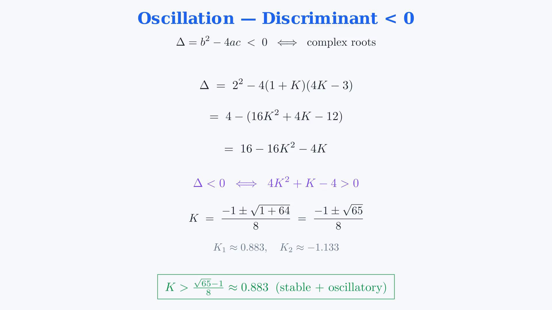
The gain three quarters is a stability boundary, and the positive discriminant boundary has a repeated real pole. Strict inequalities exclude both endpoints from their respective open intervals. Imaginary zeros are approached only as gain tends to infinity. The final example with gain ten has larger imaginary parts but real parts closer to zero than the gain-two example. Step three — oscillation.A nonreal conjugate pole pair produces sinusoidal natural modes; in the stable range here, the sinusoid is damped.Distinct real negative poles in the stable range give decaying exponential modes; a repeated real pole adds a polynomial factor, without a sinusoidal mode.The real quadratic has nonreal roots exactly when its discriminant is negative.Discriminant:Plug in.Squared linear coefficient:Product term:Expand the four a c term.Expand with the factors grouped:Group.Collect the inner terms:Expanded product:Discriminant.Subtract the entire product:Simplified discriminant:We need the discriminant strictly negative.Require sixteen minus sixteen gain squared minus four gain to be strictly negative.Multiplying by minus one reverses the inequality: sixteen gain squared plus four gain minus sixteen must be positive.After dividing by four, four gain squared plus gain minus four must be positive.Find the two boundary gains where that quadratic equals zero.Boundary gains:Square root of sixty-five is approximately eight point zero six.The boundary gains are approximately positive zero point eight eight three and negative one point one three three.The upward-opening gain quadratic is positive below the negative boundary or above the positive boundary; these decimals are approximations.Intersect the complex-pole condition with strict stability, which requires gain greater than three quarters.The lower endpoint of the strict stability interval is three quarters, and is excluded.On the stable branch, complex poles appear strictly above the positive discriminant boundary.The intersection is gain strictly above the positive exact boundary, approximately zero point eight eight three.Part c: stable oscillation requires gain strictly above the positive discriminant boundary.Exact positive boundary:Between three quarters and the positive exact boundary, excluding both endpoints, the two poles are real, distinct and negative.Narration transcript
Step three — oscillation. A second-order system oscillates when its closed-loop poles are complex — a complex conjugate pair gives a damped or undamped sinusoid in the time response. Real poles give a sum of decaying exponentials, no oscillation. The two roots of a s squared plus b s plus c equal zero are complex when the discriminant is negative. Discriminant equals b squared minus four a c. Plug in. b squared is four. Four a c is four times one plus K, times four K minus three. Expand the four a c term. Four times one plus K times four K minus three equals four times — opening the bracket — four K plus four K squared, minus three minus three K. Group. Four times four K squared plus K minus three. So four a c equals sixteen K squared plus four K minus twelve. Discriminant. Four minus the bracket. Four minus sixteen K squared minus four K plus twelve, which is sixteen minus sixteen K squared minus four K. We need the discriminant strictly negative. Sixteen minus sixteen K squared minus four K less than zero. Multiply by minus one and flip — sixteen K squared plus four K minus sixteen greater than zero. Divide by four — four K squared plus K minus four greater than zero. Solve the quadratic in K. K equals minus one, plus or minus root one plus sixty four, all over eight. Root sixty five is approximately eight point zero six. So the two roots are approximately zero point eight eight three, and minus one point one three three. The quadratic in K opens upward, so it is positive outside the roots — K less than minus one point one three three, or K greater than zero point eight eight three. Combine with stability — K greater than three quarters, that is, K greater than zero point seven five. The stability range starts at zero point seven five. The oscillation range starts at zero point eight eight three. The intersection is K greater than zero point eight eight three. Answer to question c — closed loop is oscillatory when K is greater than approximately zero point eight eight three. The exact value is root sixty five minus one, all over eight. Between zero point seven five and zero point eight eight three, the system is stable but not oscillatory — two real negative poles.
6. Follow the nonnegative-gain root locus
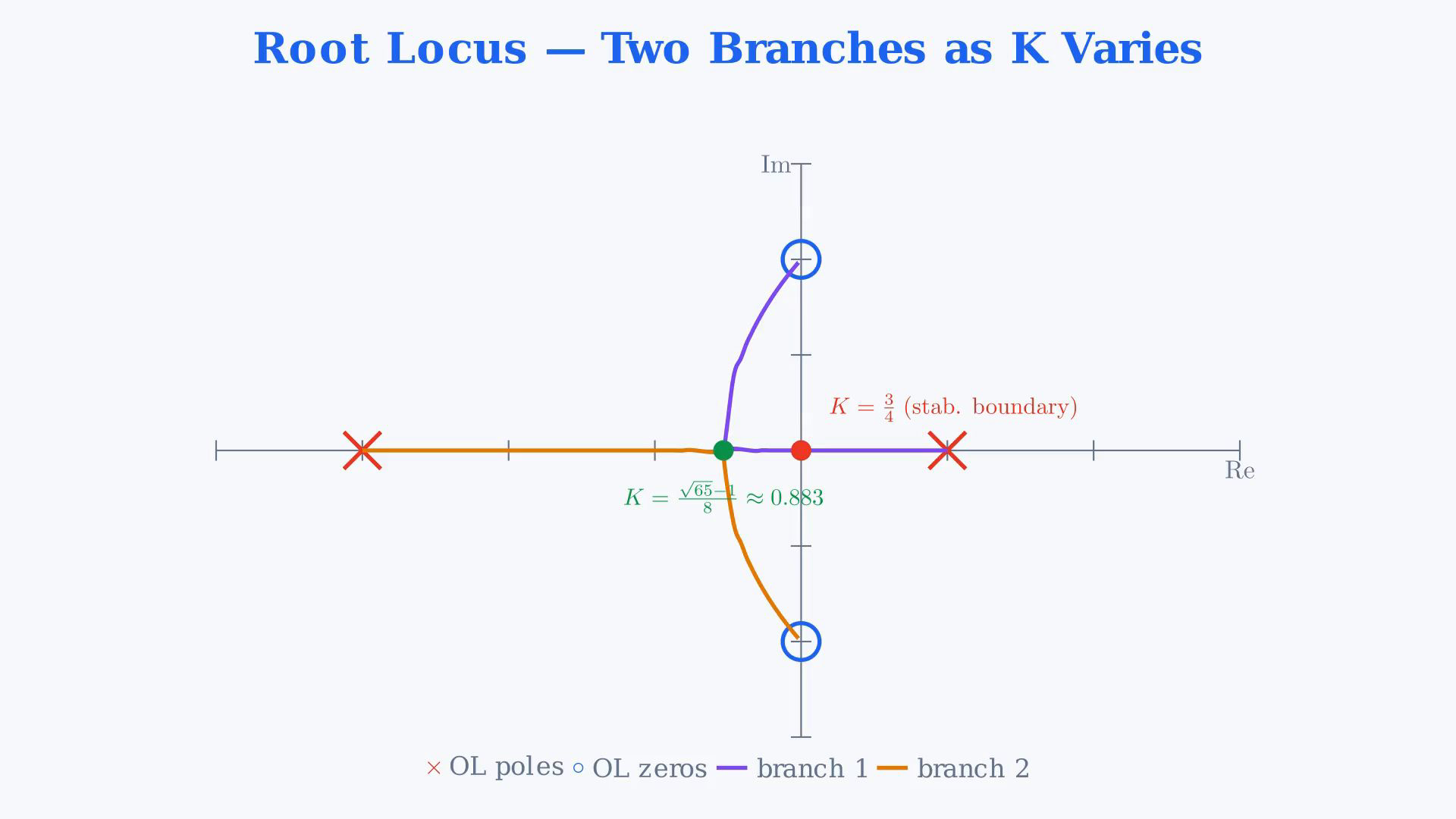
The gain three quarters is a stability boundary, and the positive discriminant boundary has a repeated real pole. Strict inequalities exclude both endpoints from their respective open intervals. Imaginary zeros are approached only as gain tends to infinity. The final example with gain ten has larger imaginary parts but real parts closer to zero than the gain-two example. Step four — root locus.Trace the closed-loop poles for nonnegative gain, from zero toward positive infinity.Rule one — number of branches.For this proper open-loop function, the branch count is its number of poles.Equal pole and zero counts:Two branches.Rule two — start and end.At the zero-gain endpoint the polynomial roots are the open-loop plant poles; equivalently these are their limits as positive gain tends to zero.As positive gain tends to infinity, the branches approach the open-loop zeros.Because pole and zero counts are equal, both branches have finite limiting zeros.Rule three — real-axis segments.Away from real poles and zeros, the positive-gain real-axis locus has an odd count of real open-loop poles and zeros to the right.Real open-loop poles:There are no real open-loop zeros; the two zeros are purely imaginary.Test the segment between the real poles.To the right of any point in this segment sits one open-loop pole — the one at plus one.Count is one.Odd.So this segment is on the locus.Test to the right of plus one.Zero open-loop poles or zeros to the right.Zero is even.Not on locus.Test to the left of minus three.Two open-loop poles to the right.Even.Not on locus.The real-axis portion including zero-gain endpoints is the interval from minus three to plus one.Rule four — asymptotes.There are no branches going to infinity and hence no root-locus asymptotes.Each branch approaches a finite zero in the infinite-gain limit.Rule five — j omega axis crossing.Substitute a purely imaginary root:Real part of the polynomial equation:Imaginary part:For finite real gain the only imaginary-axis crossing is at the origin.With zero frequency:The crossing is the strict-stability boundary, excluded from the stable interval.The picture.At zero gain, the two polynomial roots are minus three and plus one.The roots move toward one another, meet at a repeated real pole, then form a conjugate pair approaching plus and minus two j as gain tends to infinity.The origin crossing at gain three quarters is the boundary; the closed loop becomes strictly stable immediately above it.The breakaway gain is the positive exact discriminant boundary, approximately zero point eight eight three; the pair is nonreal only strictly above that gain.Narration transcript
Step four — root locus. Now sketch where the closed-loop poles travel as K varies from zero to infinity, based on the rules of root locus construction. Rule one — number of branches. The locus has max of n and m branches. Here n equals m equals two — two open-loop poles, two open-loop zeros. Two branches. Rule two — start and end. Branches start at the open-loop poles when K equals zero. Branches end at the open-loop zeros when K goes to infinity. With n equals m, every branch lands on a finite zero — no branches escape to infinity. Rule three — real-axis segments. A point on the real axis lies on the locus if and only if the total number of open-loop poles plus zeros to its right is odd. Real poles are at minus three and plus one. Real zeros — none, since the zeros are at plus or minus two j. Test the segment between the real poles. To the right of any point in this segment sits one open-loop pole — the one at plus one. Count is one. Odd. So this segment is on the locus. Test to the right of plus one. Zero open-loop poles or zeros to the right. Zero is even. Not on locus. Test to the left of minus three. Two open-loop poles to the right. Even. Not on locus. Conclusion — the real-axis portion of the locus is the segment from minus three to plus one. Rule four — asymptotes. With n minus m equals zero, there are no asymptotes. Every branch terminates at a finite zero. Rule five — j omega axis crossing. Substitute s equals j omega into the characteristic equation and solve for real K. Real part — minus one plus K times omega squared, plus four K minus three, equals zero. Imaginary part — two omega equals zero, so omega equals zero. The locus crosses the imaginary axis only at the origin. Plug omega equals zero into the real part — four K minus three equals zero — gives K equals three quarters. The crossing happens exactly at the stability boundary, consistent with question b. The picture. Two branches start at minus three and plus one on the real axis when K is zero. As K grows, they slide along the segment toward each other, meet, then break away into the complex plane and curve upward and downward, finally landing on the zeros at plus and minus two j as K goes to infinity. The locus crosses the j omega axis at the origin when K equals three quarters — that is the moment the closed loop becomes stable. The breakaway from the real axis happens at K equal to root sixty five minus one, over eight — about zero point eight eight three — the moment oscillation begins.
7. Compare boundaries and limiting poles
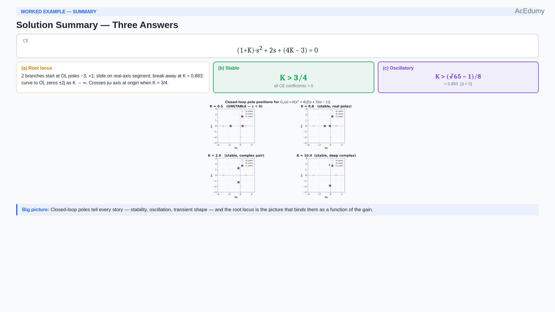
The gain three quarters is a stability boundary, and the positive discriminant boundary has a repeated real pole. Strict inequalities exclude both endpoints from their respective open intervals. Imaginary zeros are approached only as gain tends to infinity. The final example with gain ten has larger imaginary parts but real parts closer to zero than the gain-two example. Summary.Open-loop transfer function.Open-loop transfer function:Open-loop poles:Open-loop zeros:Equal counts:Closed-loop characteristic equation.Closed-loop characteristic equation:Three answers.Question a — root locus.For nonnegative gain, two branches move along the interval between the plant poles, meet at the positive discriminant boundary, and then approach the two imaginary zeros as gain tends to infinity.The finite-gain imaginary-axis crossing is at the origin, at gain three quarters.Part b: strict stability requires gain greater than three quarters.Part c: stable oscillation requires gain greater than the exact positive boundary, square root of sixty-five minus one, divided by eight.Big picture.Three questions, one characteristic equation, four short calculations.The pole locations determine modal stability and oscillation; the root locus shows their gain dependence. Zeros and residues also influence the complete transient waveform.This concludes the midterm worked-example series — twenty problems covering plant modeling, transfer functions, state space, linearization, stability, time specs, and root locus.Narration transcript
Summary. Open-loop transfer function. G sub o of s equals K times s squared plus four, divided by s plus three times s minus one. Open-loop poles at minus three and plus one. Open-loop zeros at plus and minus two j. n equals m equals two. Closed-loop characteristic equation. One plus K times s squared, plus two s, plus four K minus three, equals zero. Three answers. Question a — root locus. Two branches starting at the real poles minus three and plus one, sliding along the real-axis segment between them, breaking away at K equal to root sixty five minus one over eight, curving into the complex plane, and ending on the zeros at plus and minus two j as K grows large. The locus crosses the j omega axis at the origin when K equals three quarters. Question b — closed loop is stable when K is greater than three quarters. Question c — closed loop is oscillatory when K is greater than root sixty five minus one over eight, approximately zero point eight eight three. Big picture. Three questions, one characteristic equation, four short calculations. The closed-loop poles tell every story — stability, oscillation, transient shape — and the root locus is the picture that binds them together as a function of the gain. This concludes the midterm worked-example series — twenty problems covering plant modeling, transfer functions, state space, linearization, stability, time specs, and root locus.
Source video: Control Theory #43 — Root Locus + K Range for Stability and Oscillation (Worked Example 20) (13:57)