Control Theory · Compare Properness and Stability Using Three Routh Arrays

#35 Preserve every denominator sign, count right-half-plane roots and factor the complex conjugate poles

Compare degrees, build the quadratic and cubic Routh arrays and distinguish pole stability from minimum phase.

Question

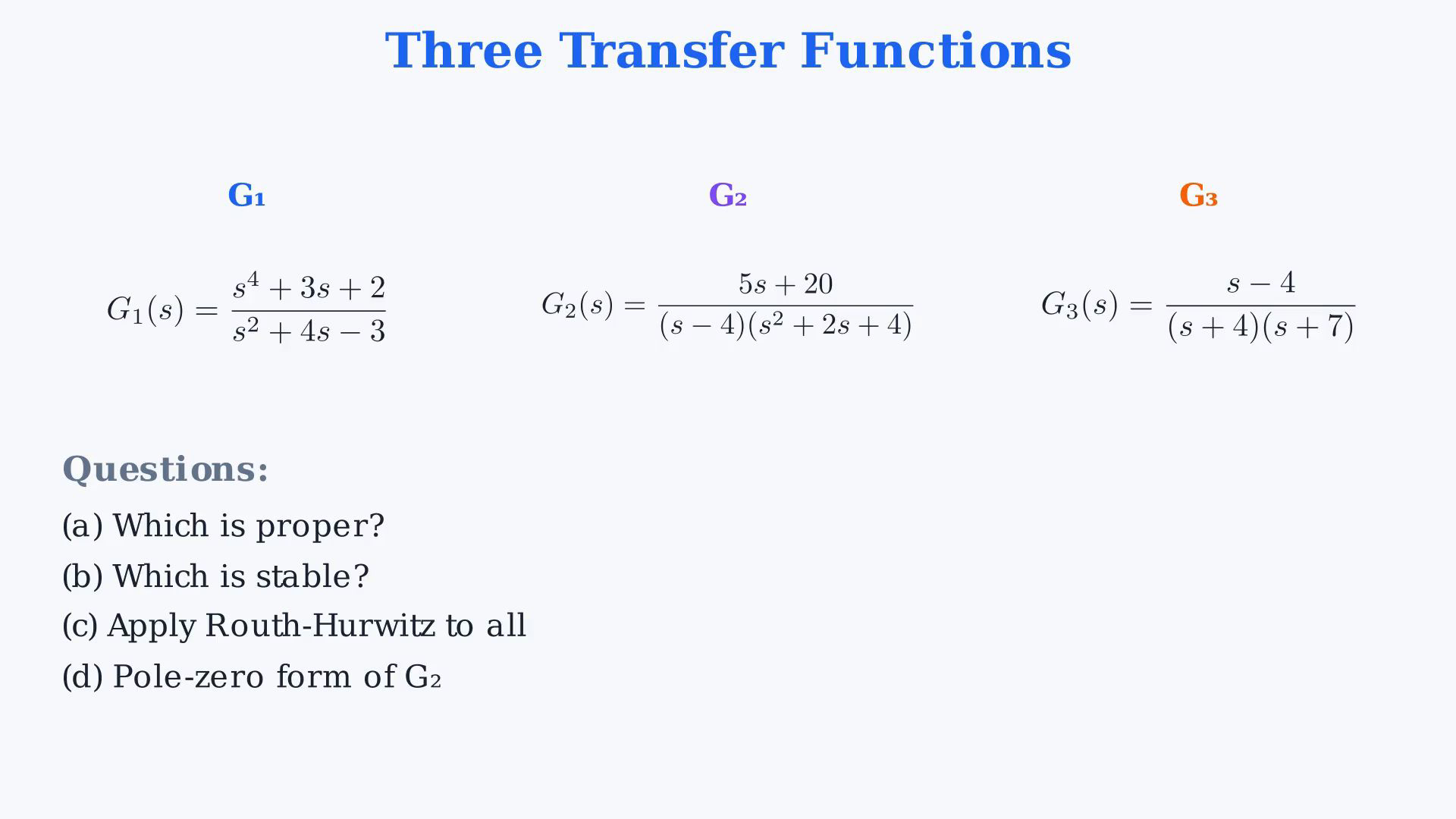
Whole existing final-video frame showing the three rational functions, their degrees, a complete Routh array or the factored pole-zero form. — Read Routh rows in descending powers of s. Sign changes are counted down the first column; they count finite right-half-plane poles after checking cancellations. Properness is a separate condition.

Analyze the three stated continuous-time real rational transfer functions: G1(s)=(s^4+3s+2)/(s²+4s-3), G2(s)=(5s+20)/[(s-4)(s²+2s+4)] and G3(s)=(s-4)/[(s+4)(s+7)]. Each full numerator and denominator must remain grouped; do not cancel opposite-sign factors such as s-4 and s+4. A transfer function is the zero-initial-condition input-output map. No physical units, hidden state realization or feedback interconnection is supplied. Properness compares polynomial degrees, not the numerical sizes of the numerator and denominator at a particular s. Let m be numerator degree and n denominator degree. Relative degree r=n-m is unchanged by a common polynomial cancellation. Proper means r>=0; strictly proper means r>0. G1 has m=4,n=2,r=-2 and is improper. G2 has m=1,n=3,r=2 and is strictly proper. G3 has m=1,n=2,r=1 and is strictly proper. Only G2 and G3 are proper. A standard finite-dimensional state-space input-output model with an ordinary bounded direct feedthrough term is proper; do not turn that into a blanket prohibition of all generalized differential or descriptor descriptions. G1 is an improper rational expression whose finite poles can still be counted. State the stability scope carefully. For a proper reduced rational continuous-time transfer function, zero-state BIBO stability holds exactly when every finite pole lies in the open left half plane. This criterion alone is not sufficient for an arbitrary improper rational expression: the ideal differentiator G(s)=s has no finite unstable poles but is not BIBO stable. Here G1 is already improper and also has one finite right-half-plane pole, so it is not BIBO stable on both grounds. G2 has a genuine pole at+4 and is unstable. G3 has poles-4 and-7 and is BIBO stable. There are no pole-zero cancellations in any of these three examples. A right-half-plane zero affects minimum phase and response shape, but does not itself destabilize a proper open-loop transfer function. Thus G3's zero+4 is compatible with its stable poles. No conclusion about a hidden nonminimal realization or a new feedback loop follows from these transfer functions alone. The spoken claim that G1 cannot be checked by inspection and needs Routh is too strong. The lesson chooses to postpone its unfactored quadratic and then practices Routh for all three. That choice is not a mathematical necessity. In fact D1(s)=s²+4s-3 has negative constant term with positive leading coefficient; its two roots have negative product and are real with opposite signs. Equivalently D1(0)<0 and D1(s) becomes positive for large positive s. The explicit roots are-2 plus or minus sqrt(7), one positive and one negative. This independent inspection agrees with the later Routh result; it does not change any coefficient, sign count or final classification. The notebook explicitly qualifies the source wording and uses the existing final summary as the overview figure rather than repeating its overstrong 'need Routh' caption. Construct each Routh array from the denominator coefficients in descending powers of s. In notebook row tuples, the first coordinate is the first column and missing coefficients are padded with zeros. For two successive rows (a,b,...) and(c,d,...) in that order from top to bottom, the next first entry is -(a*d-c*b)/c when c is nonzero. Preserve the outer minus and the entire numerator. The arrays in this exercise have no zero first-column pivots and no all-zero row. Therefore the ordinary sign-change rule applies directly; special zero-pivot or auxiliary-polynomial procedures are not needed here. In other problems, zero right-half-plane roots alone would not establish strict stability without also ruling out imaginary-axis roots. For G1, use D1=s²+4s-3. Its s² row is(1,-3), its s¹ row(4,0), and its s⁰ row(-3,0). The last first-column entry is -(1*0-4*(-3))/4=-12/4=-3. The first column(1,4,-3) has one sign change, so the quadratic has one right-half-plane root. The numerator is nonzero at both roots, so this root is a genuine pole of G1. The complete Routh result agrees with the explicit quadratic roots and with the quick sign inspection. For G2, expand D2=(s-4)(s²+2s+4)=s³+2s²+4s-4s²-8s-16=s³-2s²-4s-16. The s³ row is(1,-4), the s² row(-2,-16), the s¹ row(-12,0), and the s⁰ row(-16,0). The critical new entry is -(1*(-16)-(-2)*(-4))/(-2)=-(-16-8)/(-2)=-(-24)/(-2)=-12. In particular (-2)*(-4)=+8, and the leading minus remains outside the fraction. The first column(1,-2,-12,-16) has one sign change, between1 and-2. The following negative entries add no further sign changes. G2 therefore has exactly one right-half-plane pole, consistent with its factor s-4. For G3, D3=(s+4)(s+7)=s²+11s+28. The rows are(1,28),(11,0),(28,0) in descending powers. The last entry is -(1*0-11*28)/11=28. Its first column(1,11,28) is strictly positive with no sign changes. The explicit poles-4 and-7 additionally verify that no imaginary-axis pole is being overlooked. In the displays, v_1,v_2,v_3 denote the first-column tuples of the three arrays, and r_2,r_1,r_0 (or r_3 for the cubic) label rows by the power of s. The temporary scalars c_0 and c_1 denote a computed first-column entry for the corresponding constant or first-power row. These are calculation labels, not additional transfer functions or state vectors. Finally factor G2 completely. Its numerator5s+20=5(s+4) gives one zero at-4. The real pole is+4. For s²+2s+4, the discriminant is2²-4*1*4=-12 and the roots are(-2 plus or minus sqrt(-12))/2=-1 plus or minus j sqrt(3), with j²=-1. Over the complex numbers choose sqrt(-12)=2j sqrt(3); the plus/minus already supplies both conjugate roots. Thus G2=5(s+4)/[(s-4)(s+1-j sqrt(3))(s+1+j sqrt(3))]. The monic-factor gain is5. A pole at p contributes a denominator factor s-p, so retain the sign reversal in each complex factor. The zero-4 does not cancel the pole+4. Evaluating G2 at s=0 gives-5/4, but because the system is unstable that algebraic DC value is not a convergent unit-step steady-state output. Final-value reasoning needs its stability conditions.

Written solution and narration transcript(shows the full solution)

Below are all the lines written in the notebook together with the full narration transcript.

1. Read the three rational functions
Read Routh rows in descending powers of s. Sign changes are counted down the first column; they count finite right-half-plane poles after checking cancellations. Properness is a separate condition.
Read the problem.
Compare the three given rational functions.
First transfer function:
$\displaystyle G_{1}\left(s\right) =\frac{s^{4}+3\cdot s+2}{s^{2}+4\cdot s-3}$
Second transfer function:
$\displaystyle G_{2}\left(s\right) =\frac{5\cdot s+20}{\left(s-4\right)\cdot \left(s^{2}+2\cdot s+4\right)}$
Third transfer function:
$\displaystyle G_{3}\left(s\right) =\frac{s-4}{\left(s+4\right)\cdot \left(s+7\right)}$
First question: identify which functions are proper.
Second question: determine stability.
Third question: build all three Routh arrays.
Fourth question: factor the pole-zero form of the second function.
Narration transcript
Here is the problem. We are given three transfer functions. G1 of s equals s to the fourth plus 3 s plus 2, divided by s squared plus 4 s minus 3. G2 of s equals 5 s plus 20, divided by the quantity s minus 4 times s squared plus 2 s plus 4. G3 of s equals s minus 4, divided by the quantity s plus 4 times s plus 7. We need to answer four questions: Which transfer function is proper? Which is stable? Apply the Routh-Hurwitz method to all of them. And finally, write the pole-zero representation of G2.
2. Compare numerator and denominator degrees
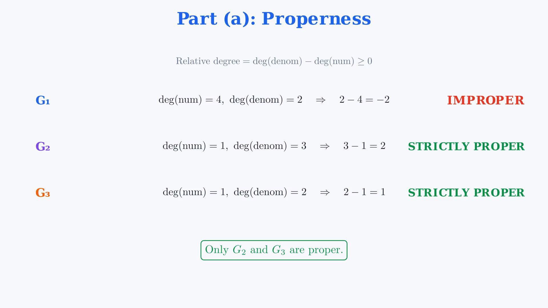
Read Routh rows in descending powers of s. Sign changes are counted down the first column; they count finite right-half-plane poles after checking cancellations. Properness is a separate condition.
Check properness.
Properness compares the numerator degree with the denominator degree.
Relative degree definition:
$\displaystyle r = n-m$
First function degrees:
$\displaystyle m = 4; n = 2$
First relative degree:
$\displaystyle r = 2-4 = -2$
The first function is improper because its numerator degree is larger.
Second function degrees:
$\displaystyle m = 1; n = 3$
Second relative degree:
$\displaystyle r = 3-1 = 2$
The second function is strictly proper.
Third function degrees:
$\displaystyle m = 1; n = 2$
Third relative degree:
$\displaystyle r = 2-1 = 1$
The third function is strictly proper.
Only the second and third functions are proper.
Narration transcript
Part a: which transfer function is proper? A transfer function is proper when the degree of the numerator is less than or equal to the degree of the denominator. The relative degree equals denominator degree minus numerator degree, and it must be greater than or equal to zero. For G1, the numerator has degree 4 and the denominator has degree 2. Relative degree equals 2 minus 4, which is negative 2. G1 is improper, the numerator is bigger than the denominator. For G2, the numerator has degree 1 and the denominator has degree 3. Relative degree equals 3 minus 1, which is 2. G2 is strictly proper. For G3, the numerator has degree 1 and the denominator has degree 2. Relative degree equals 2 minus 1, which is 1. G3 is strictly proper. Conclusion: only G2 and G3 are proper.
3. Inspect the poles and state the stability scope
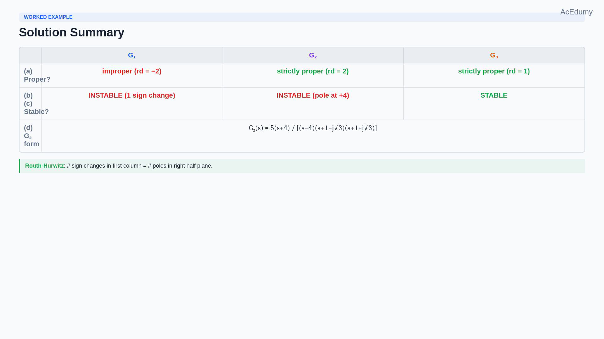
Read Routh rows in descending powers of s. Sign changes are counted down the first column; they count finite right-half-plane poles after checking cancellations. Properness is a separate condition.
Inspect the poles before building the arrays.
For proper reduced rational transfer functions, all finite poles must have strictly negative real parts for BIBO stability.
Unfactored first denominator:
$\displaystyle D_{1}\left(s\right) = s^{2}+4\cdot s-3$
The source chooses Routh here; its negative constant term also lets us detect a positive root by inspection.
Second denominator:
$\displaystyle D_{2}\left(s\right) = \left(s-4\right)\cdot \left(s^{2}+2\cdot s+4\right)$
A factor with this sign gives:
$\displaystyle p_{1} = 4$
The second function is unstable because its pole at positive four is not canceled.
Third denominator:
$\displaystyle D_{3}\left(s\right) = \left(s+4\right)\cdot \left(s+7\right)$
Third function poles:
$\displaystyle p_{1} = -4; p_{2} = -7$
The third function is proper with both poles strictly in the left half plane, so it is BIBO stable.
Build all three full Routh arrays to practice the method.
Narration transcript
Part b: a quick stability check by inspection. A transfer function is stable when all poles have strictly negative real parts, meaning all poles lie in the open left half plane. For G1, the denominator s squared plus 4 s minus 3 is not factored. We cannot tell stability by inspection here, we will need the Routh-Hurwitz method. For G2, the denominator is already factored as s minus 4 times s squared plus 2 s plus 4. The factor s minus 4 gives a pole at s equals positive 4. This pole is in the right half plane, so G2 is instable, no calculation needed. For G3, the denominator is s plus 4 times s plus 7. The poles are at s equals negative 4 and s equals negative 7. Both have negative real parts, so G3 is stable. Even though we already know G2 and G3 by inspection, we will still build the full Routh table for all three to practice the method.
4. Build the first quadratic Routh table
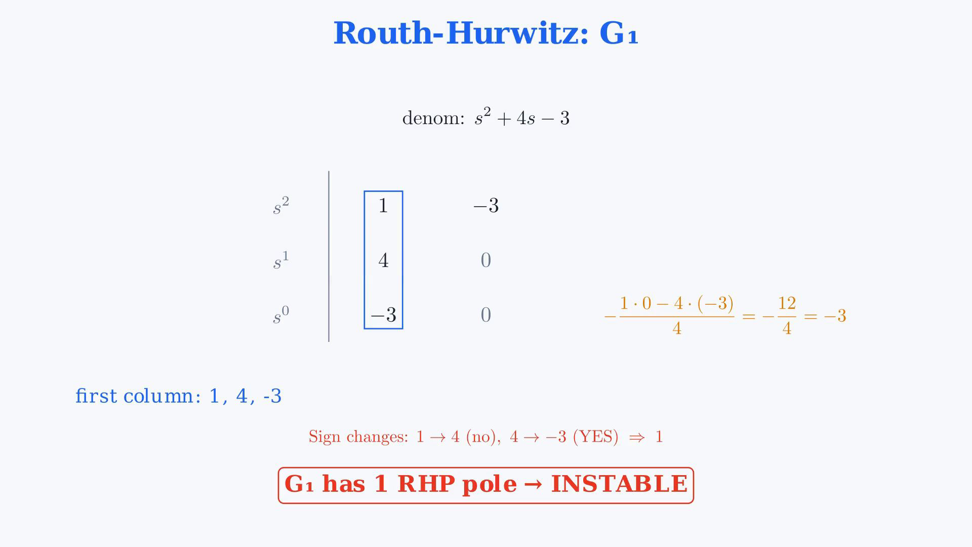
Read Routh rows in descending powers of s. Sign changes are counted down the first column; they count finite right-half-plane poles after checking cancellations. Properness is a separate condition.
Build the Routh array for the first function.
Quadratic denominator:
$\displaystyle D_{1}\left(s\right) = s^{2}+4\cdot s-3$
The quadratic array has three rows.
Row for the square power:
$\displaystyle r_{2} = \left(1,-3\right)$
Row for the first power:
$\displaystyle r_{1} = \left(4,0\right)$
Compute the constant row.
Preserve the outer minus, the determinant order and the divisor from the row above.
Constant-row first entry:
$\displaystyle c_{0} = -\frac{1\cdot 0-4\cdot \left(-3\right)}{4}$
Simplify the entry:
$\displaystyle -\frac{12}{4 }= -3$
First column:
$\displaystyle v_{1} = \left(1,4,-3\right)$
Count changes in sign down this column.
One to four stays positive.
Four to minus three changes sign once.
Sign-change count:
$\displaystyle N_{\mathrm{RHP}} = 1$
With no special zero rows or pivots here, the sign-change count equals the number of right-half-plane denominator roots.
The first function has one uncanceled right-half-plane pole and is unstable.
Narration transcript
Part c: Routh-Hurwitz for G1. The denominator is s squared plus 4 s minus 3, a second order polynomial. The Routh array has three rows. The s squared row uses the first and third coefficients: 1 and minus 3. The s one row uses the second coefficient: 4, padded with zero. For the s zero row, we use the standard formula. The first column entry is the determinant of the two by two block above, with a minus sign in front, divided by the leading entry of the row above. We get minus the quantity 1 times zero minus 4 times minus 3, divided by 4. That is minus 12 over 4, which equals minus 3. The first column reads: 1, 4, minus 3. We count the sign changes. From 1 to 4, no change. From 4 to minus 3, one sign change. Total: 1 sign change. By the Routh-Hurwitz criterion, the number of poles in the right half plane equals the number of sign changes. So G1 has 1 unstable pole and is instable, confirming what we suspected.
5. Expand the cubic and count sign changes
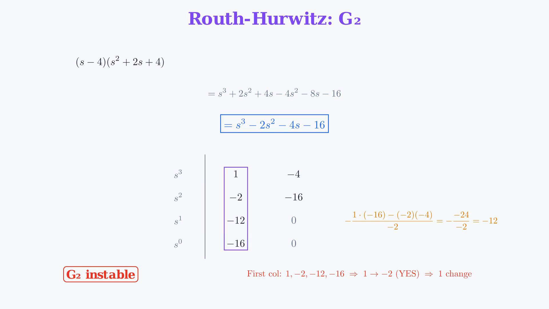
Read Routh rows in descending powers of s. Sign changes are counted down the first column; they count finite right-half-plane poles after checking cancellations. Properness is a separate condition.
Build the Routh array for the second function.
First expand its factored denominator.
Factored denominator:
$\displaystyle D_{2}\left(s\right) = \left(s-4\right)\cdot \left(s^{2}+2\cdot s+4\right)$
Multiply the factors:
$\displaystyle D_{2}\left(s\right) = s^{3}+2\cdot s^{2}+4\cdot s-4\cdot s^{2}-8\cdot s-16$
Combine powers:
$\displaystyle D_{2}\left(s\right) = s^{3}-2\cdot s^{2}-4\cdot s-16$
The cubic array has four rows.
Row for the cube power:
$\displaystyle r_{3} = \left(1,-4\right)$
Row for the square power:
$\displaystyle r_{2} = \left(-2,-16\right)$
First-power row entry:
$\displaystyle c_{1} = -\frac{1\cdot \left(-16\right)-\left(-2\right)\cdot \left(-4\right)}{-2}$
Evaluate the product in the numerator:
$\displaystyle c_{1} = -\frac{-16-8}{-2}$
Keep the outer minus:
$\displaystyle -\frac{-24}{-2}= -12$
Constant row:
$\displaystyle r_{0} = \left(-16,0\right)$
First column:
$\displaystyle v_{2} = \left(1,-2,-12,-16\right)$
One to minus two changes sign once.
Minus two to minus twelve stays negative.
Minus twelve to minus sixteen stays negative.
Sign-change count:
$\displaystyle N_{\mathrm{RHP}} = 1$
The second function has one unstable pole, agreeing with the visible positive-four factor.
Narration transcript
Routh-Hurwitz for G2. First, we expand the factored denominator. S minus 4, times s squared plus 2 s plus 4. Multiplying out: s cubed plus 2 s squared plus 4 s, minus 4 s squared minus 8 s minus 16. Combining like terms: s cubed minus 2 s squared minus 4 s minus 16. Now we build the Routh table for this third order polynomial. The s cubed row uses the first and third coefficients: 1 and minus 4. The s squared row uses the second and fourth coefficients: minus 2 and minus 16. For the s one row, the formula gives minus the quantity 1 times minus 16 minus minus 2 times minus 4, divided by minus 2. That is minus the quantity minus 16 minus 8, divided by minus 2. Which is minus minus 24 over minus 2, equal to minus 12. The s zero row carries down minus 16. The first column reads: 1, minus 2, minus 12, minus 16. Count sign changes: 1 to minus 2, one sign change. Minus 2 to minus 12, no change. Minus 12 to minus 16, no change. Total: 1 sign change. G2 has 1 unstable pole, confirming the pole at positive 4 we saw by inspection.
6. Build the stable quadratic Routh table
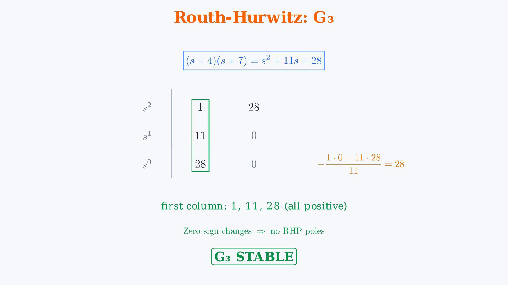
Read Routh rows in descending powers of s. Sign changes are counted down the first column; they count finite right-half-plane poles after checking cancellations. Properness is a separate condition.
Build the Routh array for the third function.
Factored denominator:
$\displaystyle D_{3}\left(s\right) = \left(s+4\right)\cdot \left(s+7\right)$
Expand the denominator:
$\displaystyle D_{3}\left(s\right) = s^{2}+11\cdot s+28$
The quadratic array again has three rows.
Row for the square power:
$\displaystyle r_{2} = \left(1,28\right)$
Row for the first power:
$\displaystyle r_{1} = \left(11,0\right)$
Constant-row first entry:
$\displaystyle c_{0} = -\frac{1\cdot 0-11\cdot 28}{11}$
Simplified entry:
$\displaystyle r_{0} = \left(28,0\right)$
First column:
$\displaystyle v_{3} = \left(1,11,28\right)$
All first-column entries are positive.
Sign-change count:
$\displaystyle N_{\mathrm{RHP}} = 0$
This third denominator has no right-half-plane roots.
The known negative real poles also rule out imaginary-axis roots; the third function is stable.
Narration transcript
Routh-Hurwitz for G3. The denominator is s plus 4 times s plus 7. Expanding gives s squared plus 11 s plus 28. Building the Routh table for this second order polynomial. The s squared row: 1 and 28. The s one row: 11 and zero. For the s zero row, the formula gives minus the quantity 1 times zero minus 11 times 28, divided by 11. That simplifies to 28. The first column reads: 1, 11, 28. All three values are positive. Zero sign changes. By Routh-Hurwitz, G3 has zero unstable poles. G3 is stable, confirming the negative real poles we found.
7. Factor the numerator and complex pole pair
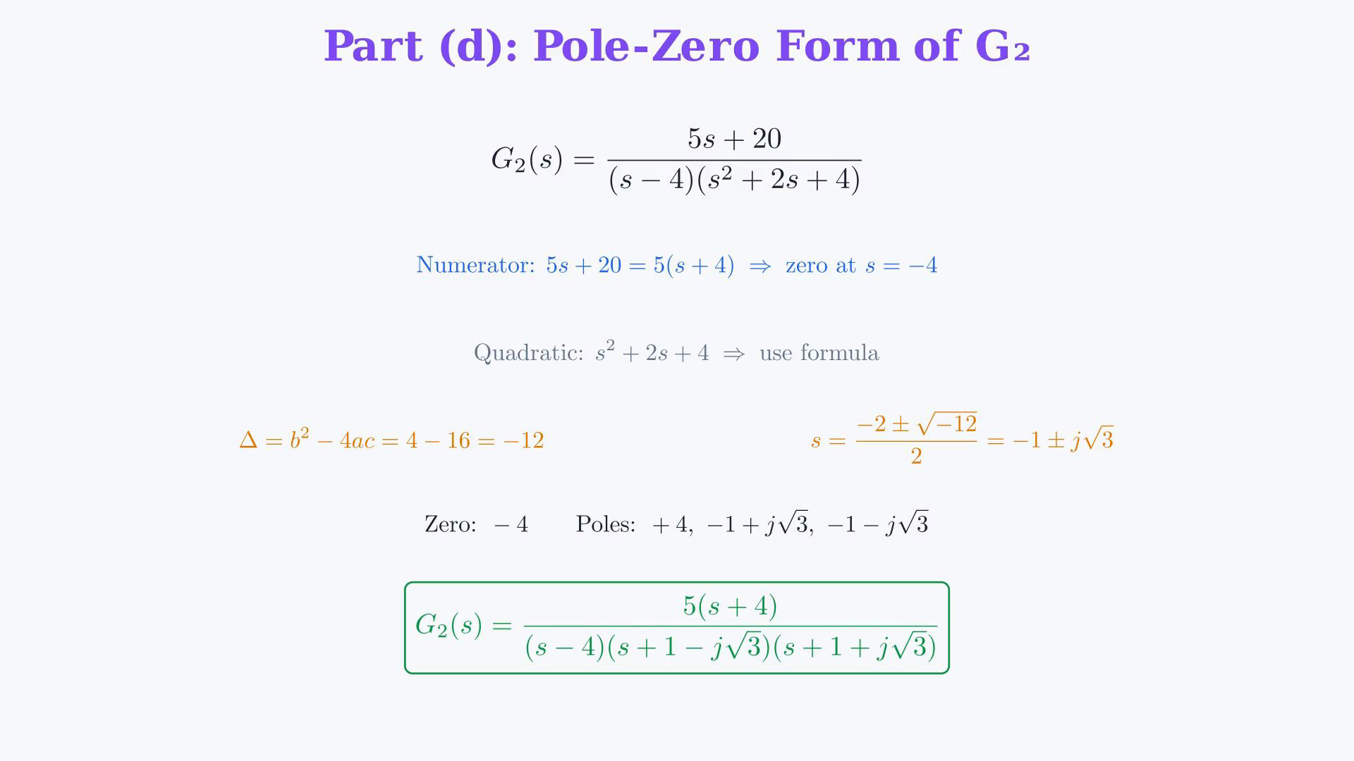
Read Routh rows in descending powers of s. Sign changes are counted down the first column; they count finite right-half-plane poles after checking cancellations. Properness is a separate condition.
Write the pole-zero form of the second function.
Identify every finite zero and pole.
Start from the original expression:
$\displaystyle G_{2}\left(s\right) =\frac{5\cdot s+20}{\left(s-4\right)\cdot \left(s^{2}+2\cdot s+4\right)}$
Factor the numerator:
$\displaystyle 5\cdot s+20 = 5\cdot \left(s+4\right)$
Single zero:
$\displaystyle z_{1} = -4$
Real pole:
$\displaystyle p_{1} = 4$
Apply the quadratic formula to the remaining second-order factor.
Discriminant:
$\displaystyle \Delta = 2^{2}-4\cdot 1\cdot 4 = 4-16 = -12$
Quadratic roots over the complex numbers:
$\displaystyle s =\frac{-2\pm \sqrt{-12}}{2}$
Simplify the conjugate roots:
$\displaystyle s = -1\pm j\cdot \sqrt{3}$
All three poles:
$\displaystyle p_{1} = 4; p_{2} = -1+j\cdot \sqrt{3}; p_{3} = -1-j\cdot \sqrt{3}$
Complete factored form:
$\displaystyle G_{2}\left(s\right) = 5\cdot \frac{s+4}{\left(s-4\right)\cdot \left(s+1-j\cdot \sqrt{3}\right)\cdot \left(s+1+j\cdot \sqrt{3}\right)}$
Narration transcript
Part d: pole-zero representation of G2. We need to find all the zeros and all the poles of G2 explicitly. G2 of s equals 5 s plus 20, divided by s minus 4 times s squared plus 2 s plus 4. First, factor the numerator: 5 s plus 20 equals 5 times s plus 4. So G2 has a single zero at s equals minus 4. For the poles, we already have one factor s minus 4, giving a pole at s equals 4. For the quadratic s squared plus 2 s plus 4, we use the quadratic formula. The discriminant is b squared minus 4 a c, equal to 4 minus 16, which is minus 12. The roots are s equals minus 2 plus or minus the square root of minus 12, all divided by 2. That gives s equals minus 1 plus or minus j square root of 3. So G2 has three poles total: positive 4, minus 1 plus j root 3, and minus 1 minus j root 3. The pole-zero form is: G2 of s equals 5 times s plus 4, divided by s minus 4 times s plus 1 minus j root 3 times s plus 1 plus j root 3.
8. Compare the three results
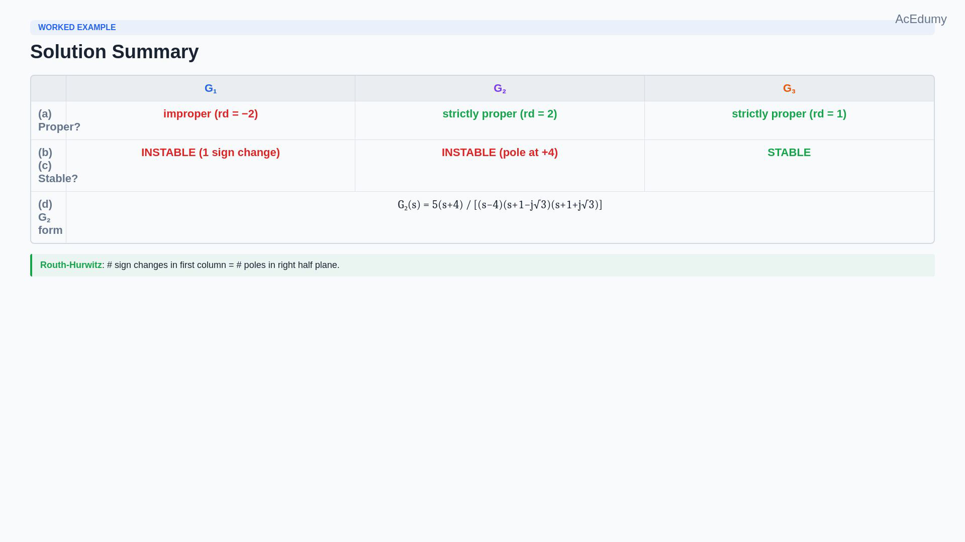
Read Routh rows in descending powers of s. Sign changes are counted down the first column; they count finite right-half-plane poles after checking cancellations. Properness is a separate condition.
Review all three functions.
Keep properness, pole stability and the Routh count distinct.
The first function is improper with relative degree minus two and one right-half-plane pole.
The second function is strictly proper with relative degree two but has a pole at positive four.
The third function is strictly proper with relative degree one and has only left-half-plane poles.
Second function zero and poles:
$\displaystyle z_{1} = -4; p_{1} = 4; p_{2} = -1+j\cdot \sqrt{3}; p_{3} = -1-j\cdot \sqrt{3}$
The four requested parts are complete.
Narration transcript
Let us recap. We analyzed three transfer functions for properness, stability, and the Routh criterion. G1 is improper with relative degree minus 2, and instable with one right-half-plane pole. G2 is strictly proper with relative degree 2, but instable due to the pole at positive 4. G3 is strictly proper with relative degree 1, and stable, all poles in the open left half plane. And the pole-zero form of G2: numerator zero at minus 4, denominator poles at positive 4, and minus 1 plus or minus j root 3. Four parts done, Routh-Hurwitz analysis complete.