Control Theory · Second-Order Step Response

#13 Classify the zero-state step response of a standard second-order lag by damping ratio and pole geometry

Relate damping ratio to real, repeated and complex poles, then compare overdamped, critical, oscillatory and unstable step responses.

Question

Existing lesson frame showing a standard second-order transfer, pole classification or response curve. — Use the standard constant-numerator second-order lag with positive T and the stated zero initial conditions. The introduction, underdamped explanation and pole geometry use the clean pole-classification card as an algebraic reference. Response graphs use normalized time t/T and output y/K with K=1; the family graph clips excursions outside its displayed vertical range and does not model saturation.

Use the standard continuous-time LTI second-order lag with constant numerator K, positive natural time constant T and zero initial output and derivative. Its ODE is T squared times y double prime plus 2 D T times y prime plus y equals K times u. The natural angular frequency is 1/T, the damping ratio D is dimensionless and K is the DC transfer gain. This is a particular zero-free second-order model, not every second-order transfer function: numerator zeros or other input-output channels can change overshoot and initial behavior. Two independent energy-storage states are a common physical realization, not a requirement that every abstract second-order equation contain two literal circuit elements. For nonzero K the transfer denominator has no cancellation. If K is zero the zero-state transfer vanishes while an ODE initial-state mode may remain. Use a causal unit step sigma(t); its isolated value at zero does not affect the response formulas here. The step response starts with y(0)=0 and right derivative zero. For nonzero initial output or derivative add the corresponding homogeneous solution; the zero-state transfer alone omits those terms. For positive T the characteristic roots are minus D plus or minus the square root of D squared minus one, all divided by T. When D exceeds one both poles are distinct negative reals. When D is one the pole is repeated at minus 1/T. Stable underdamping requires D strictly between zero and one. Complex poles more generally occur for D strictly between minus one and one; it is false to infer complex poles for every D below one. At D zero there are simple poles at plus and minus j/T and undamped free oscillations. This boundary is not asymptotically stable and is not BIBO stable: a resonant bounded sinusoid can produce unbounded output. At D minus one there is a repeated positive real pole; below minus one both poles are positive real and the instability need not oscillate. Every negative D yields an unstable dynamic mode; distinguish this from a vanishing K input-output channel. For D greater than one define T1=T times (D plus square root of D squared minus one) and T2=T times (D minus that square root). Then T1 and T2 are positive, their sum is 2DT and product T squared, and the denominator factors into (1+T1 s)(1+T2 s). The step response contains the constant final term K plus two decaying exponential transients, not merely two exponentials that both vanish to zero. For nonzero K its normalized output is one minus T1/(T1-T2) times exp(-t/T1) plus T2/(T1-T2) times exp(-t/T2), for nonnegative t. For positive K it rises monotonically without overshoot; negative K reverses the direction. Keeping T, K, step amplitude and initial-state convention fixed, increasing D above one slows the dominant mode. It moves one pole toward the origin even though the other moves farther left. At D one the transfer denominator is the square of the whole factor one plus T s. The causal step response is K times [one minus (one plus t/T) times exp(-t/T)] times sigma(t). Keep both nested groups and the minus exponent. The response approaches K asymptotically, never reaching the exact final value at a finite positive time for nonzero K. Fastest non-oscillatory means the fastest monotonic member of this zero-state, zero-free family when T and K are fixed and D is at least one. It is not a universal fastest response across different natural frequencies, initial conditions, numerator zeros or settling tolerances. For stable underdamping define omega_d=square root of (1-D squared) divided by T and phi=arccos(D). Then the normalized positive-time step response is one minus exp(-Dt/T)/square root of (1-D squared) times sin(omega_d t plus phi). This phase choice enforces the two zero initial conditions. The fractional overshoot is exp(-pi D/square root of (1-D squared)); smaller positive D gives a larger overshoot and slower exponential envelope when T stays fixed. This does not establish a statistical claim that underdamping is the most common real-system behavior; treat that narration as motivation only. The family graph compares D=1.5,1,0.7,0.4,0.1 and -0.1 at fixed normalization. Its displayed vertical range clips the unstable excursions; do not read edge segments as physical saturation or finite bounds. The normalized final reference is one; the source K reference corresponds to K=1. For the upper stable complex pole, the angle arccos(D) is measured from the negative real axis about the origin, not from the positive real axis. The pole magnitude is 1/T and its real part is minus D/T. Pole geometry describes modal decay rates and frequencies. Poles alone do not specify gain, residues, numerator zeros, excitation or initial-state amplitudes and do not reveal everything about a general system. Within a minimal proper rational input-output model, all poles strictly in the left half-plane establish BIBO stability; internal stability additionally requires the relevant internal modes. Simple nonzero imaginary-axis poles give persistent free sinusoids here, whereas repeated imaginary-axis poles can produce polynomial growth and a pole at the origin is not itself a sinusoid. More negative real part means a faster exponential decay of that mode, not an unconditional faster total step response if other poles, residues or zeros change. D controls the normalized damping character, T sets the time scale and K sets output scale; none is dispensable in predicting the full response. These results support later controller design but do not themselves provide a controller or tracking guarantee.

Written solution and narration transcript(shows the full solution)

Below are all the lines written in the notebook together with the full narration transcript.

1. Introduce second-order responses
Use the standard constant-numerator second-order lag with positive T and the stated zero initial conditions. The introduction, underdamped explanation and pole geometry use the clean pole-classification card as an algebraic reference. Response graphs use normalized time t/T and output y/K with K=1; the family graph clips excursions outside its displayed vertical range and does not model saturation.
Introduce Control Theory, Lesson 13.
Recall the first-order step response.
Study a standard second-order lag with two independent dynamic states.
Use D to classify the normalized damping behavior.
Connect this response family to its characteristic poles.
Narration transcript
Welcome to lesson thirteen. In the previous lesson we studied step responses for first-order systems. Now we move to the second-order lag, a system with two energy storage elements. The damping ratio D determines whether the response is smooth, critically damped, or oscillatory. By the end of this lesson, you will understand all three cases and how pole locations in the s-plane control the behavior.
2. Derive the zero-state transfer
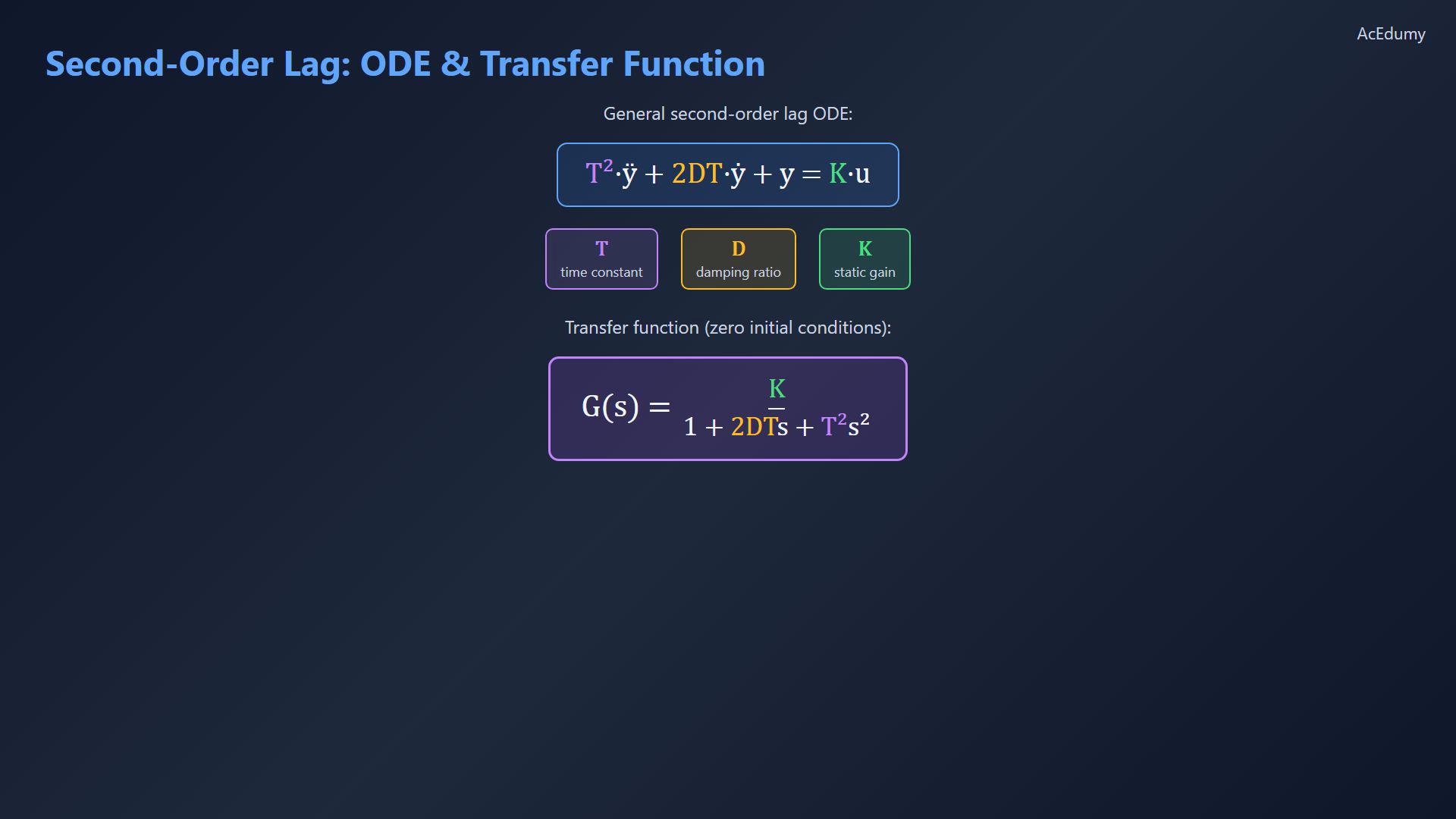
Use the standard constant-numerator second-order lag with positive T and the stated zero initial conditions. The introduction, underdamped explanation and pole geometry use the clean pole-classification card as an algebraic reference. Response graphs use normalized time t/T and output y/K with K=1; the family graph clips excursions outside its displayed vertical range and does not model saturation.
Standard lag ODE:
$\displaystyle T²\cdot y''\left(t\right) + 2\cdot D\cdot T\cdot y'\left(t\right) + y\left(t\right) = K\cdot u\left(t\right)$
Define positive T, dimensionless damping D and constant DC gain K.
Zero-initial-state transfer:
$\displaystyle G\left(s\right) =\frac{ K}{1+2\cdot D\cdot T\cdot s+T²\cdot s²}$
Narration transcript
The general second-order lag is described by the ODE: T squared times y double-dot, plus 2 D T times y dot, plus y, equals K times u. Here T is the natural time constant, D is the damping ratio, and K is the static gain. Taking the Laplace transform with zero initial conditions gives the transfer function: G of s equals K, divided by one plus 2 D T s plus T squared s squared.
3. Classify the two poles
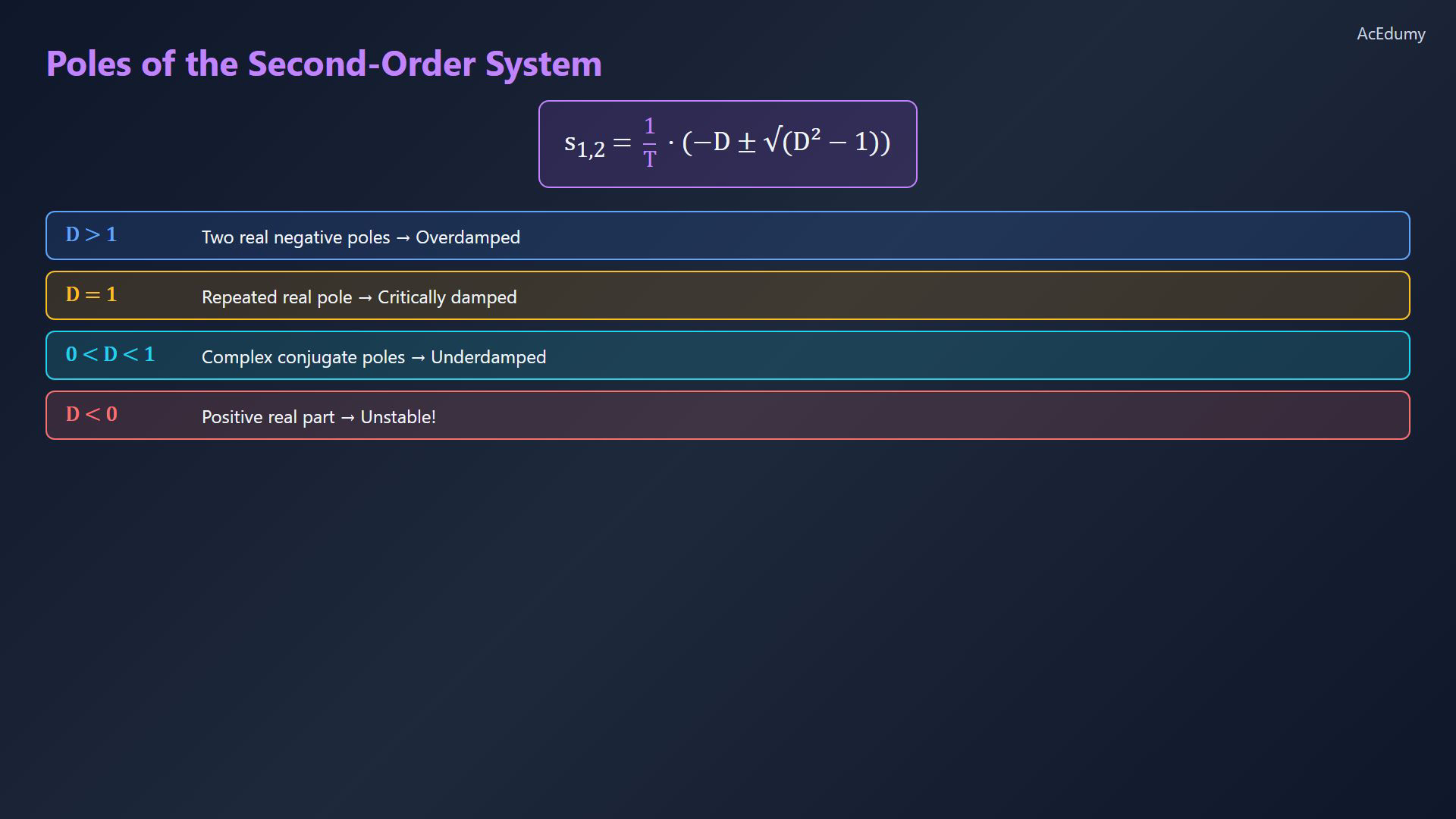
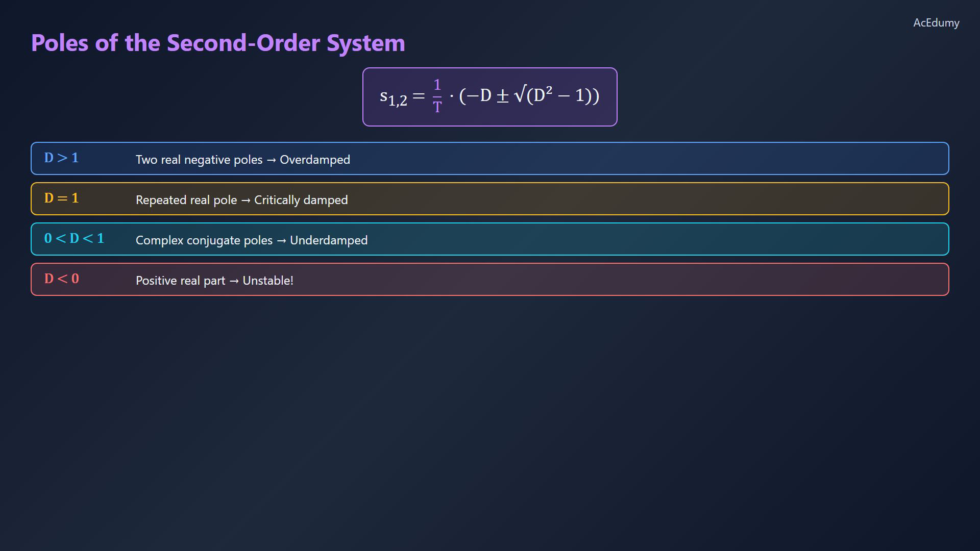
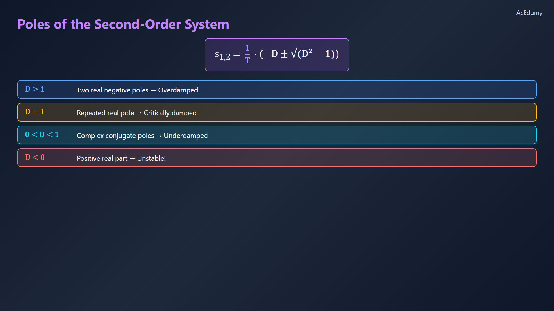
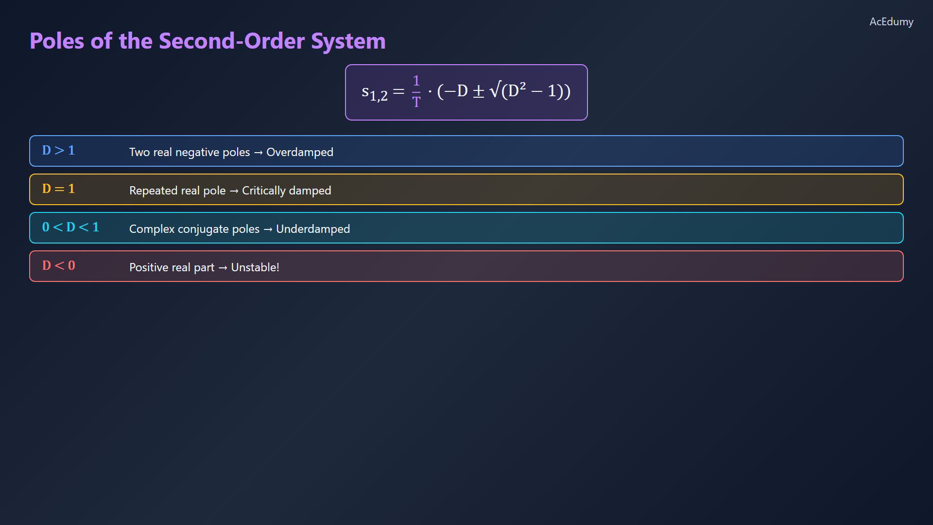
Use the standard constant-numerator second-order lag with positive T and the stated zero initial conditions. The introduction, underdamped explanation and pole geometry use the clean pole-classification card as an algebraic reference. Response graphs use normalized time t/T and output y/K with K=1; the family graph clips excursions outside its displayed vertical range and does not model saturation.
Characteristic roots:
$\displaystyle s_{1,2} = \left(\frac{1}{T}\right)\cdot \left(-D \pm \sqrt{D²-1}\right)$
Classify both roots with positive T.
For D greater than one, both roots are real and negative.
At D equal to one, the negative real pole is repeated.
For D strictly between zero and one, the poles form a stable complex pair.
Negative D gives positive real parts and an unstable dynamic mode.
Narration transcript
The denominator zeros, which are the poles, are s one two equals one over T, times negative D plus or minus the square root of D squared minus one. The value of D determines the pole type. When D is greater than one, both poles are real and negative, meaning stable. When D equals one, we get a repeated real pole. When D is between zero and one, the poles are complex conjugates. And when D is negative, at least one pole has a positive real part, and the system is unstable.
4. Factor the overdamped lag
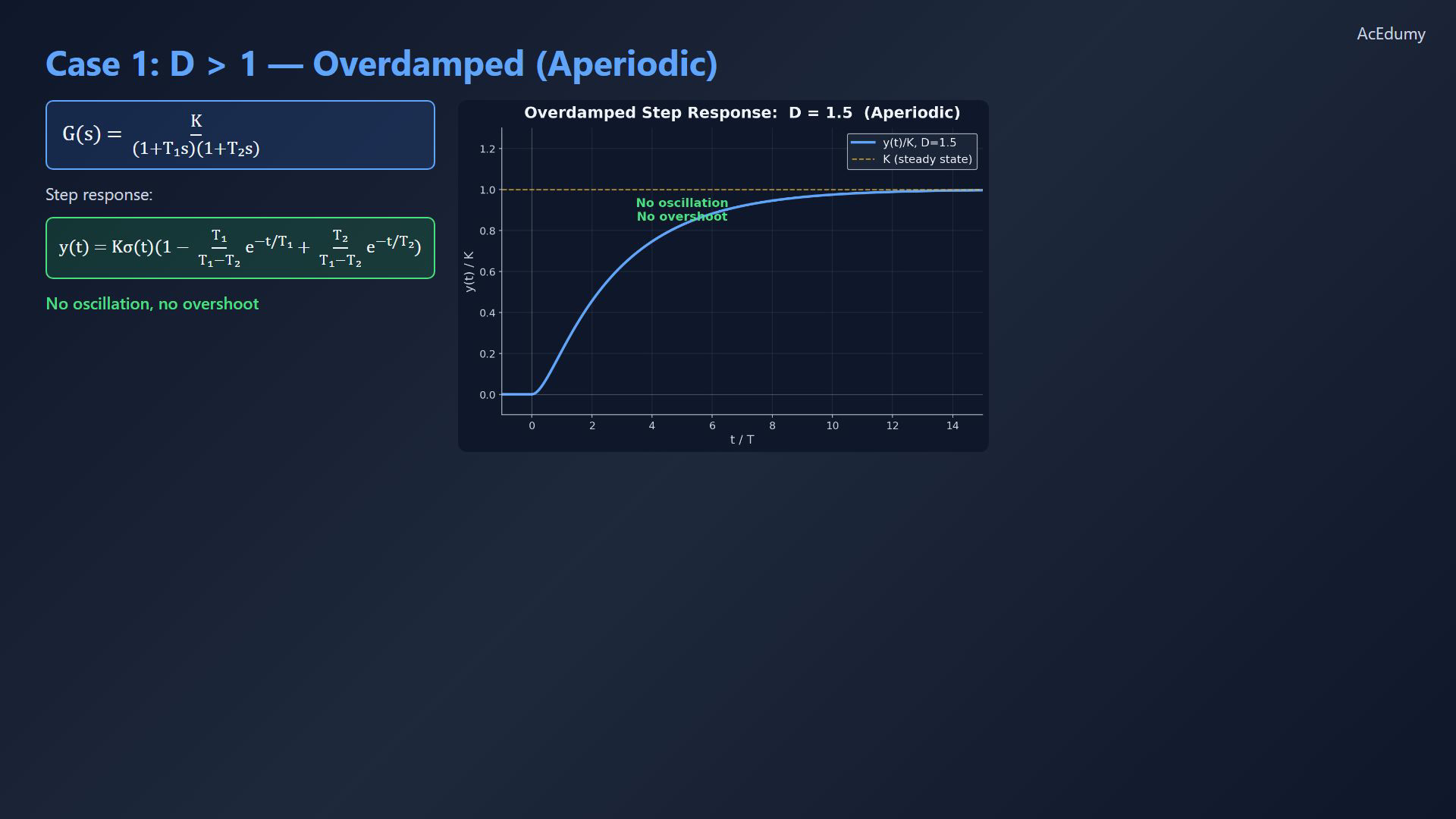
Use the standard constant-numerator second-order lag with positive T and the stated zero initial conditions. The introduction, underdamped explanation and pole geometry use the clean pole-classification card as an algebraic reference. Response graphs use normalized time t/T and output y/K with K=1; the family graph clips excursions outside its displayed vertical range and does not model saturation.
Overdamped factorization:
$\displaystyle G\left(s\right) =\frac{ K}{\left(1+T_{1}\cdot s\right)\cdot \left(1+T_{2}\cdot s\right)}$
Include the constant final term K plus two decaying exponential transients.
This zero-state standard lag does not oscillate.
For positive K, approach K monotonically without overshoot.
Call the D-greater-than-one case overdamped or aperiodic.
At fixed T and gain, larger overdamping slows the dominant response.
Narration transcript
When D is greater than one, the transfer function factors into two first-order lags: G of s equals K divided by the product of one plus T one s, times one plus T two s. The step response is a sum of two decaying exponentials. There is no oscillation. The output rises smoothly toward K and never overshoots. This is called the aperiodic or overdamped case. The larger D is, the slower the response.
5. Check critical damping
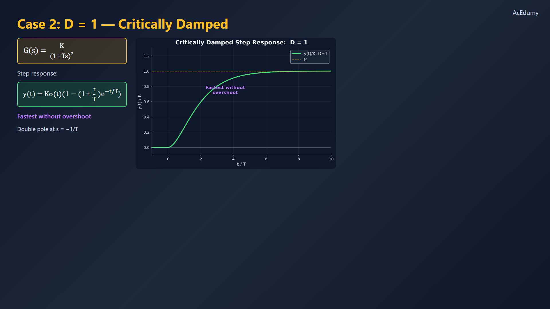
Use the standard constant-numerator second-order lag with positive T and the stated zero initial conditions. The introduction, underdamped explanation and pole geometry use the clean pole-classification card as an algebraic reference. Response graphs use normalized time t/T and output y/K with K=1; the family graph clips excursions outside its displayed vertical range and does not model saturation.
Repeated critical pole:
$\displaystyle s_{1} = s_{2} = -\frac{1}{T}$
Critical transfer:
$\displaystyle G\left(s\right) =\frac{ K}{\left(1+T\cdot s\right)^{2}}$
Critical step response:
$\displaystyle y\left(t\right) = K\cdot \left(1-\left(1+\frac{t}{T}\right)\cdot e^{-t/T}\right)\cdot \sigma \left(t\right)$
At fixed T, this is the fastest monotonic member of the stated zero-state lag family.
Approach K asymptotically without overshoot.
D equal to one separates the stable overdamped and underdamped cases.
Narration transcript
When D equals exactly one, the two poles merge into a double pole at s equals negative one over T. The transfer function becomes G of s equals K divided by one plus T s, all squared. The step response is y of t equals K times one minus one plus t over T, times e to the negative t over T. This is the fastest non-oscillatory response. It reaches K without overshooting, but just barely. It marks the boundary between overdamped and underdamped behavior.
6. Describe the underdamped response
Use the standard constant-numerator second-order lag with positive T and the stated zero initial conditions. The introduction, underdamped explanation and pole geometry use the clean pole-classification card as an algebraic reference. Response graphs use normalized time t/T and output y/K with K=1; the family graph clips excursions outside its displayed vertical range and does not model saturation.
Stable underdamping requires D strictly between zero and one.
The transient contains a sinusoid with a decaying exponential envelope.
For nonzero K, oscillate about the final value with decreasing amplitude.
At fixed T, smaller positive D gives larger fractional overshoot.
Use this as a model of damped oscillation, not a universal frequency claim about real systems.
Narration transcript
When D is between zero and one, the poles become complex conjugates. The step response contains a damped sinusoid. The output oscillates around K with decreasing amplitude. Smaller D means more oscillation and larger overshoot. This underdamped case is the most common in practice, because many real systems have some degree of oscillation before settling to their final value.
7. Compare damping ratios
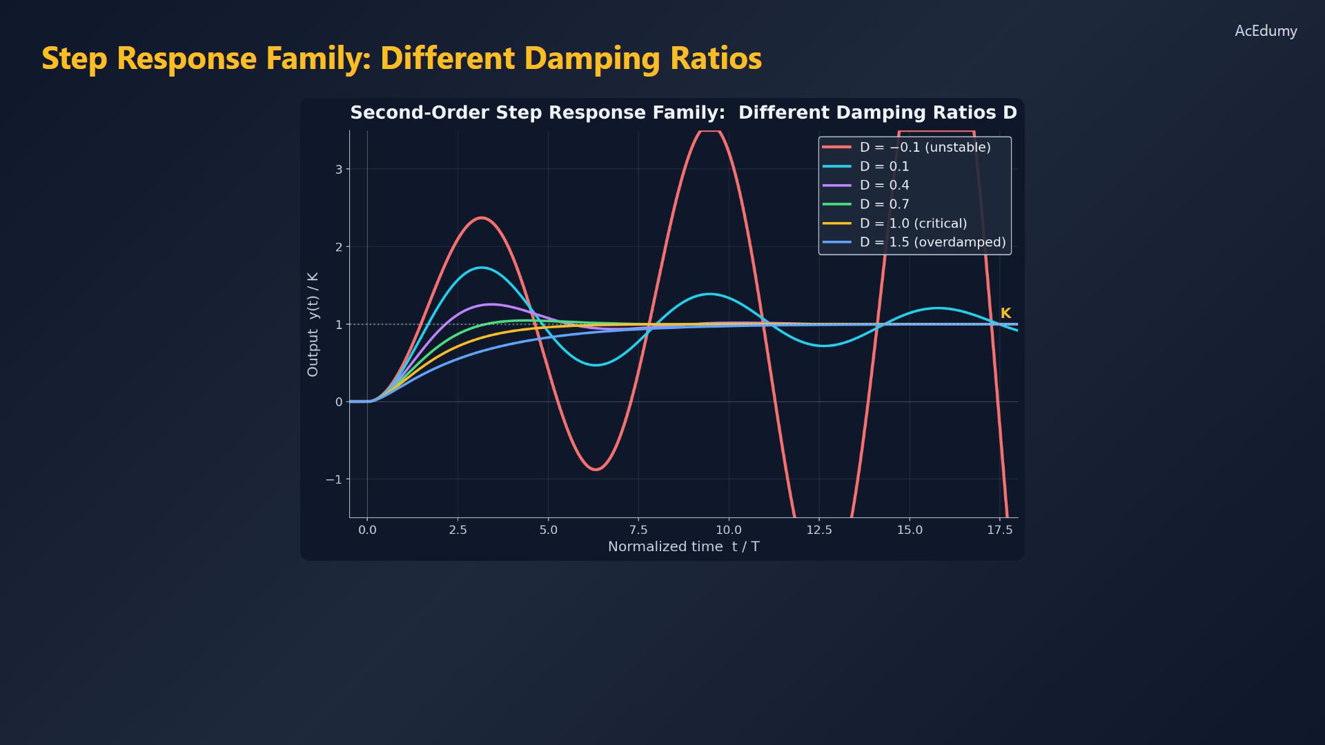
Use the standard constant-numerator second-order lag with positive T and the stated zero initial conditions. The introduction, underdamped explanation and pole geometry use the clean pole-classification card as an algebraic reference. Response graphs use normalized time t/T and output y/K with K=1; the family graph clips excursions outside its displayed vertical range and does not model saturation.
Compare the response family at fixed normalized time and gain.
D of 1.5 gives a slow monotonic overdamped response.
D of 1 gives the critical monotonic response.
D of 0.7 gives a small overshoot.
D of 0.4 gives a larger overshoot and visible oscillation.
D of 0.1 gives stronger oscillation with a slowly decaying envelope.
D of negative 0.1 gives growing oscillation; excursions exceed the plotted vertical range.
D sets damping character; retain T for time scale and K for output scale.
Narration transcript
Let us compare all cases on one graph. For D equals 1.5, the overdamped response rises slowly with no oscillation. For D equals 1, the critically damped case is faster but still no overshoot. For D equals 0.7, a slight overshoot appears. For D equals 0.4, stronger oscillation with significant overshoot. For D equals 0.1, heavy oscillation that takes a long time to settle. And for D equals negative 0.1, the system is unstable, and the oscillations grow without bound. The damping ratio D is the single most important parameter for second-order systems.
8. Read the pole geometry
Use the standard constant-numerator second-order lag with positive T and the stated zero initial conditions. The introduction, underdamped explanation and pole geometry use the clean pole-classification card as an algebraic reference. Response graphs use normalized time t/T and output y/K with K=1; the family graph clips excursions outside its displayed vertical range and does not model saturation.
Use poles to describe modal rates and frequencies; gain and initial state still matter.
For D greater than one, both roots lie on the negative real axis.
For D equal to one, the pole is repeated.
For stable underdamping, use the range strictly between zero and one.
Angle from the negative real axis:
$\displaystyle \varphi = \arccos \left(D\right)$
For the specified minimal rational channel, poles strictly in the left half-plane imply BIBO stability.
The D-zero boundary has persistent free oscillation and lacks BIBO stability.
Right-half-plane dynamic poles imply instability.
A more negative real part makes that mode decay faster; compare all modes for the full response.
Narration transcript
The pole locations in the s-plane reveal everything about system behavior. When D is greater than one, two poles sit on the negative real axis. When D equals one, they merge into a double pole. When D is less than one, the poles become complex conjugates forming an angle with the real axis. This angle equals arccosine of D. Poles in the left half-plane guarantee stability. Poles on the imaginary axis produce sustained oscillation. And poles in the right half-plane cause instability. The further left the poles, the faster the response decays.
9. Review the classification scope
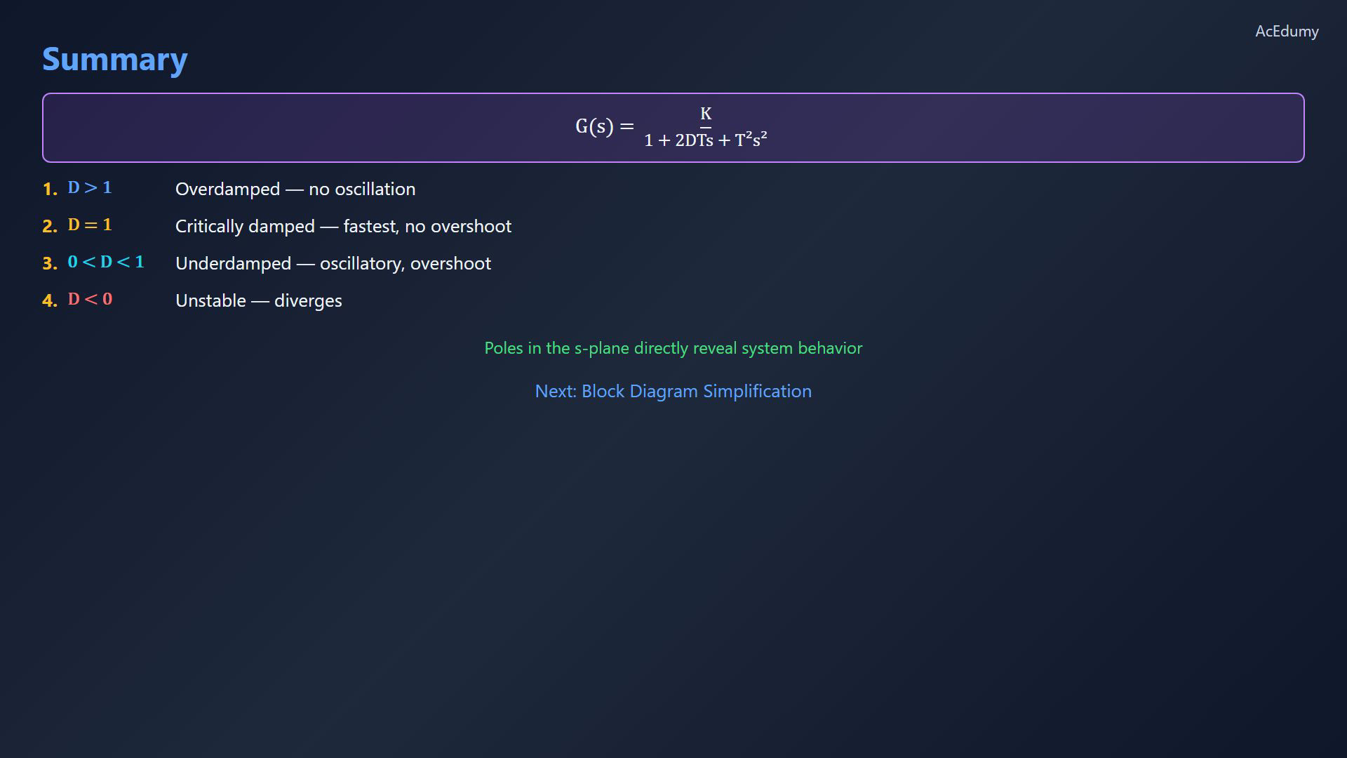
Use the standard constant-numerator second-order lag with positive T and the stated zero initial conditions. The introduction, underdamped explanation and pole geometry use the clean pole-classification card as an algebraic reference. Response graphs use normalized time t/T and output y/K with K=1; the family graph clips excursions outside its displayed vertical range and does not model saturation.
Review the standard second-order lag.
Transfer form:
$\displaystyle G\left(s\right) =\frac{ K}{1+2\cdot D\cdot T\cdot s+T²\cdot s²}$
D controls normalized damping behavior.
D greater than one gives the stable overdamped case.
D equal to one gives critical damping at the stated fixed time scale.
Stable underdamping and overshoot require D strictly between zero and one.
D below zero gives an unstable dynamic mode.
Use pole geometry together with gain, model scope and initial conditions.
Apply these model properties when studying controller design.
Continue with block diagram simplification.
Narration transcript
Let us summarize. The second-order lag has transfer function K over one plus 2 D T s plus T squared s squared. The damping ratio D controls the character of the response. D greater than one gives overdamped behavior with no oscillation. D equals one is critically damped, the fastest without overshoot. D less than one is underdamped, oscillatory with overshoot. And D less than zero means instability. The poles in the s-plane directly reveal the system behavior. This understanding is fundamental for controller design. Next, we will study block diagram simplification.