Control Theory · Separate Internal Stability, BIBO Stability and a Cubic Routh Test

#37 Trace the unreachable stable mode and handle a zero Routh pivot without dividing by zero

Derive the zero-state transfer function, identify the canceled mode and count two unstable roots of the separate cubic using an infinitesimal pivot.

Question

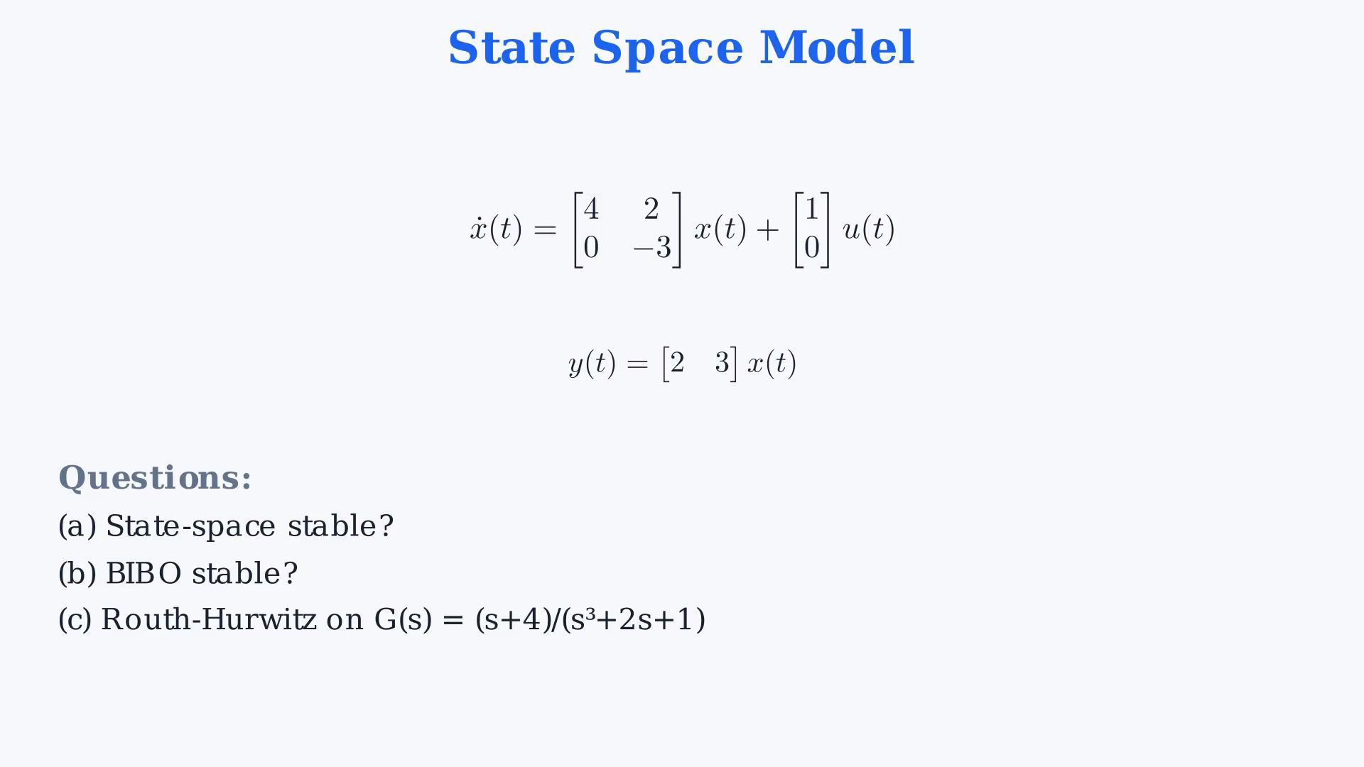
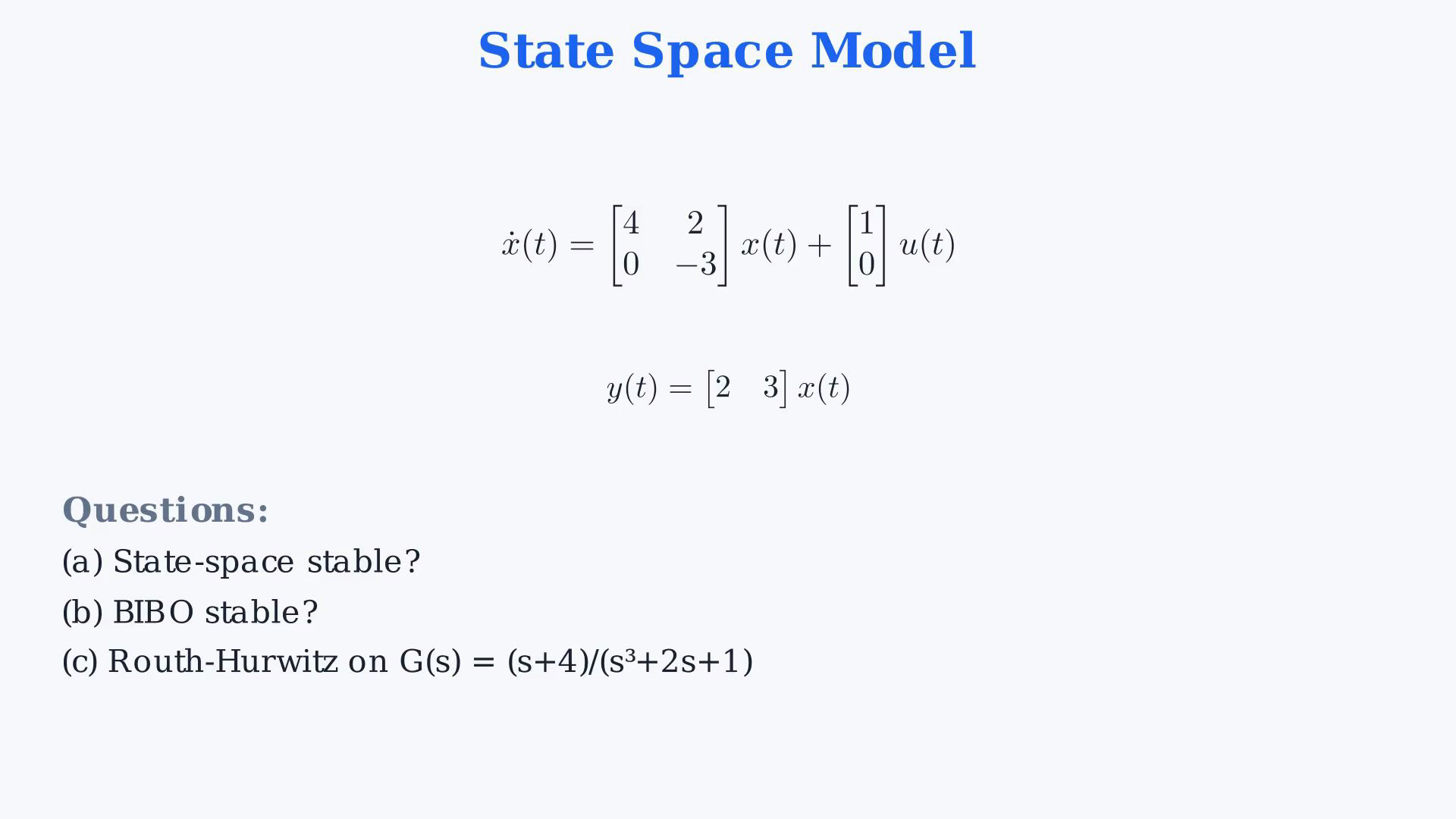
Whole existing final-video frame showing the state matrices, complete resolvent derivation, canceled factor, cubic coefficient ordering, epsilon Routh table or final comparison. — The state model and the cubic transfer function are separate problems. In the Routh figure, negative infinity records a one-sided limit; for every small positive epsilon the actual entry is finite.

Answer three stability questions. The continuous-time state model has A with first row(4,2) and second row(0,-3), input column b=(1,0)transpose, and output row ctranspose=(2,3), with xprime=A*x+b*u and y=ctranspose*x. There is no direct feedthrough term. Equivalently x1prime=4x1+2x2+u, x2prime=-3x2, y=2x1+3x2. Part(a) concerns internal stability of this state model. Part(b) concerns its zero-state bounded-input bounded-output map. Part(c) is a different transfer function (s+4)/(s³+2s+1). To distinguish the two functions that the source calls G, the notebook labels the part(b) function G_b and the part(c) function G_c; this is only a label, not a new interconnection. No feedback design, physical units or nonzero initial-state transfer-function formula is supplied. For part(a), the strict left-half-plane eigenvalue criterion is for internal asymptotic (equivalently exponential, for finite-dimensional LTI models) stability. Merely bounded Lyapunov stability can allow semisimple imaginary-axis eigenvalues; do not erase that distinction by reading every use of stable as the same property. Here A is upper triangular, so its eigenvalues are4 and-3. The positive eigenvalue4 proves instability even in the weaker Lyapunov sense. For example with zero input and initial state(1,0)transpose, the state is(exp(4t),0)transpose and grows. No root calculation based only on the transfer function can remove that internal eigenvalue. For part(b), BIBO means every bounded input produces a bounded zero-state output. With this ordinary finite-dimensional state model and zero direct term, the transfer function is strictly proper. For a proper reduced real rational transfer function, zero-state BIBO stability is equivalent to every finite pole lying strictly in the open left half plane. The source uses the transfer-function route; an equivalent direct impulse-response calculation from the state model is also possible. A's eigenvalues alone are not enough to infer the exact poles when a realization is nonminimal. For zero initial state G_b(s)=ctranspose*(sI-A)^(-1)*b. The resolvent expression is first evaluated away from A's eigenvalues, then simplified as a rational function. Let M(s)=sI-A. Its first row is(s-4,-2) and its second row(0,s+3). Define d(s)=det(M)=(s-4)(s+3)-(-2)*0=(s-4)(s+3). The inverse has first row((s+3)/d,2/d) and second row(0,(s-4)/d). Preserve the negative2 in M and positive2 in its adjugate. For readability the displays use M_1,M_2 for the two rows of M; A_1,A_2 for the two rows of A; R_1,R_2 for the two rows of M^(-1); and J_1,J_2 for the two rows of the adjugate. These are row tuples in the stated order, not column vectors or extra state variables. The input b is a column, and the display btranspose=(1,0) specifies that column unambiguously. Let q(s)=M^(-1)b be a column. Since b selects the first inverse column, q1=(s+3)/d and q2=0. Multiplying the output row gives G_b=2q1+3q2=2(s+3)/[(s-4)(s+3)]. The factor s+3 cancels in the input-output rational expression, leaving G_b=2/(s-4). It removes the transfer-function pole at-3, but the remaining pole+4 is genuine. Thus the map is not BIBO stable. Its impulse response is2exp(4t) for t>=0; the bounded unit step gives y=(exp(4t)-1)/2 from rest, which is an explicit unbounded-output witness. Identify why the-3 mode disappears here instead of assigning a generic cancellation cause without checking. The controllability matrix[b,Ab] has rows(1,4),(0,0), so its rank is1: the reachable subspace is the first coordinate axis. Starting from rest, x2 remains zero for every input because x2prime=-3x2 has no input term. The eigenmode-3 is unreachable from b. It is observable: the observability matrix has rows ctranspose=(2,3) and ctranspose*A=(8,-5), whose determinant is-34, so its rank is2. An eigenvector for-3 is(-2/7,1)transpose and its output projection is17/7, nonzero. In general a canceled mode may be unreachable, unobservable or both; this particular example is unreachable and observable. The canceled mode here is stable. The summary's statement that cancellations can hide unstable internal modes is a general possibility, not a claim that this canceled-3 mode is unstable. Algebraic cancellation does not delete the state from the physical realization or suppress the response to a nonzero initial condition. For part(c), use only G_c=(s+4)/(s³+0*s²+2s+1). Its numerator zero is-4, while the denominator there is-71, so it cancels no root. List all coefficients, including the zero quadratic coefficient. The first Routh row, labeled s³, is(1,2); the second, labeled s², is(0,1). This is a zero first-column pivot with another nonzero entry in the row. It is not an all-zero row and does not call for the auxiliary-polynomial method. Replace only that zero pivot by epsilon>0 and examine the limit epsilon→0 from above. This positive infinitesimal is a calculation device; it is not a finite design change to the supplied system. With the replacement the rows are(1,2),(epsilon,1),(2-1/epsilon,0),(1,0) in descending powers of s. The new s¹ entry is (epsilon*2-1*1)/epsilon=(2epsilon-1)/epsilon=2-1/epsilon. Its numerator remains grouped over the same epsilon. For every0<epsilon<1/2, this entry is negative and finite. The final first-column entry follows from the Routh formula as[(2-1/epsilon)*1-epsilon*0]/(2-1/epsilon)=1. As epsilon→0+, the third entry tends to negative infinity. The figure's-∞ records this limiting sign, not a finite row entry on which to perform arithmetic or a value of a pole. The first-column sign sequence is positive,positive,negative,positive, giving exactly two sign changes. An arbitrary large positive replacement would be invalid: for example epsilon=1 changes the sign count. The one-sided infinitesimal limit is essential. The sign count gives two denominator roots in the open right half plane, both uncanceled, so this separate transfer function is unstable. No imaginary-axis root is hidden: substituting s=jw gives real part1 for every real w. Independently, the original real cubic P(s)=s³+2s+1 has derivative3s²+2>0 and exactly one real root r between-1/2 and0. Dividing by s-r gives the quadratic s²+r*s+(r²+2). Its discriminant-3r²-8 is negative, and its conjugate pair has real part-r/2>0. This confirms exactly two right-half-plane roots without relying on epsilon arithmetic. Hidden in the Routh explanation means revealed by handling the zero pivot; these two poles are not canceled input-output modes. The outcomes are: an internally unstable state model, its non-BIBO input-output map with one pole+4, and a separate cubic map with two right-half-plane poles.

Written solution and narration transcript(shows the full solution)

Below are all the lines written in the notebook together with the full narration transcript.

1. Read the state model and the separate cubic problem
The state model and the cubic transfer function are separate problems. In the Routh figure, negative infinity records a one-sided limit; for every small positive epsilon the actual entry is finite.
Read the problem.
Use the given two-state model.
State equation:
$\displaystyle x' = A\cdot x+b\cdot u$
Rows of the system matrix:
$\displaystyle A_{1} = \left(4,2\right); A_{2} = \left(0,-3\right)$
Input column specified by its transpose:
$\displaystyle b^{T} = \left(1,0\right)$
Output equation:
$\displaystyle y = 2\cdot x_{1}+3\cdot x_{2}$
Answer three distinct questions.
Part a: test internal asymptotic stability of this state model.
Part b: test the bounded-input bounded-output map from zero state.
Part c is a separate function:
$\displaystyle G_{c}\left(s\right) =\frac{s+4}{s^{3}+2\cdot s+1}$
Narration transcript
Here is the problem. We are given a state space model. The state derivative x-dot equals the matrix A times the state x plus the vector b times the input u. Here A is a 2 by 2 matrix with rows 4 and 2 in the first row, and 0 and negative 3 in the second row. The input vector b is 1 and 0. The output y equals c transpose x, where c transpose is 2 and 3. We need to answer three questions. Part a: Is the state space model stable? Part b: Is the system BIBO stable? Part c: For a different transfer function, G of s equals s plus 4, divided by s cubed plus 2 s plus 1, apply the Routh-Hurwitz criterion.
2. Test internal asymptotic stability from the eigenvalues
The state model and the cubic transfer function are separate problems. In the Routh figure, negative infinity records a one-sided limit; for every small positive epsilon the actual entry is finite.
Test internal stability of the state model.
Strictly negative eigenvalue real parts characterize internal asymptotic stability for this finite-dimensional LTI model.
The characteristic roots come from the determinant of the resolvent matrix.
The lower-left entry is zero, so the matrix is upper triangular.
Triangular-matrix eigenvalues are its diagonal entries.
The diagonal entries are four and minus three.
Eigenvalues:
$\displaystyle \lambda _{1} = 4; \lambda _{2} = -3$
The first eigenvalue is positive.
It lies in the open right half plane.
The positive mode grows under zero input, so the state model is unstable.
Narration transcript
Part a: check internal stability of the state space model. A state space system is stable when all eigenvalues of A have strictly negative real parts. To find the eigenvalues, we would normally compute the determinant of s I minus A. But here A is upper triangular — the lower-left entry is zero. For a triangular matrix, the eigenvalues are simply the diagonal entries. The diagonal entries are 4 and negative 3. So the eigenvalues of A are lambda 1 equals 4 and lambda 2 equals negative 3. The eigenvalue 4 has positive real part. That is in the right half plane. Conclusion: the state space model is INSTABLE.
3. Define the zero-state BIBO test
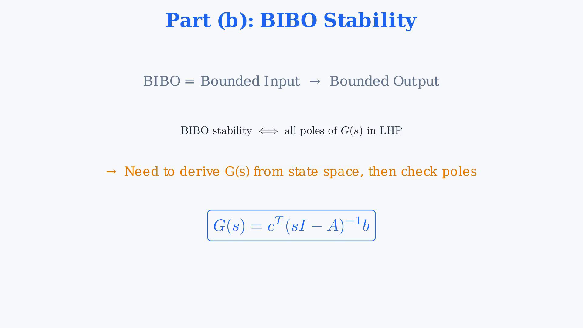
The state model and the cubic transfer function are separate problems. In the Routh figure, negative infinity records a one-sided limit; for every small positive epsilon the actual entry is finite.
Test BIBO stability of the input-output map.
BIBO means bounded input, bounded output.
Every bounded input must produce a bounded zero-state output.
For a proper reduced rational transfer function, check its poles; a nonminimal state model can contain additional modes.
Derive the transfer function here and then inspect its remaining poles.
Zero-state transfer function with no direct term:
$\displaystyle G_{b}\left(s\right) = c^{T}\cdot \left(s\cdot I-A\right)^{-1}\cdot b$
Compute the resolvent and matrix products step by step.
Narration transcript
Part b: check BIBO stability. BIBO stands for Bounded Input Bounded Output. A system is BIBO stable if every bounded input produces a bounded output. BIBO stability is determined by the transfer function, not directly by the state space model. We need to derive the transfer function from the state space, then check its poles. The formula is G of s equals c transpose times the inverse of s I minus A, all times b. Let us compute this step by step.
4. Compute the resolvent and transfer function
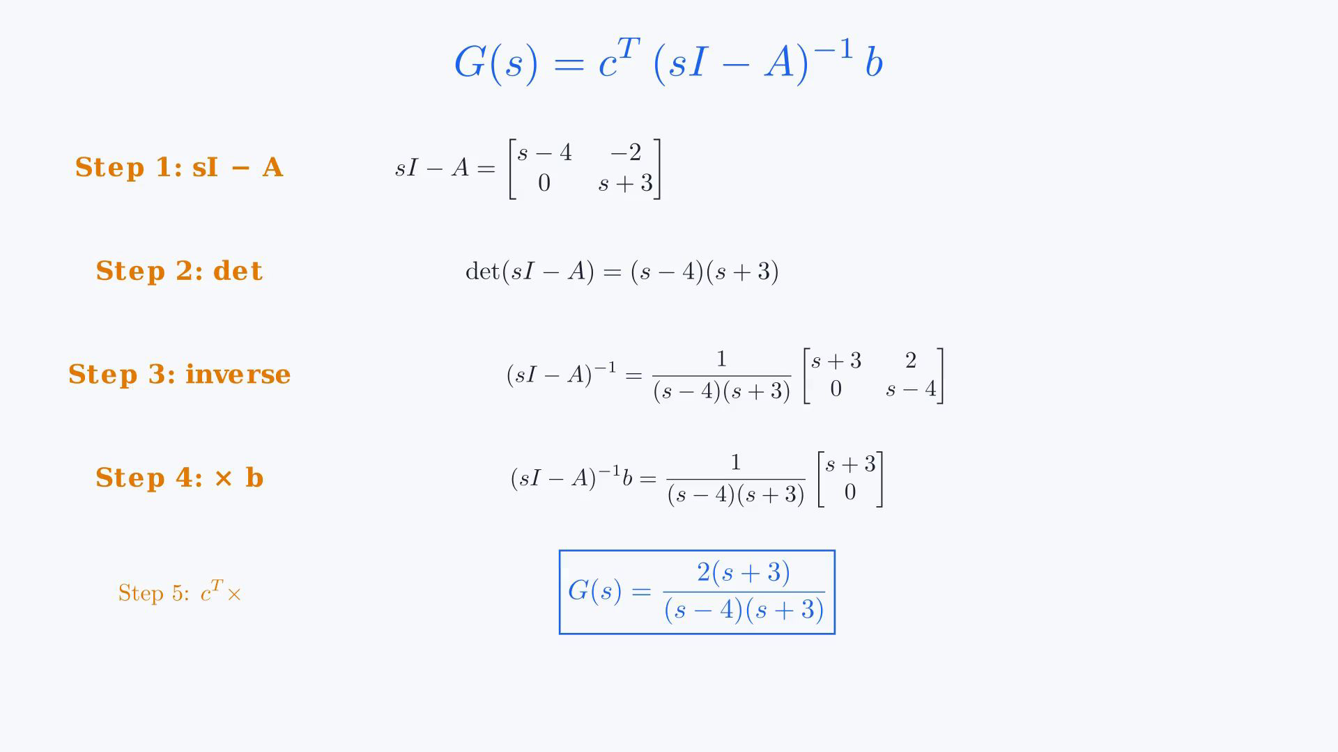
The state model and the cubic transfer function are separate problems. In the Routh figure, negative infinity records a one-sided limit; for every small positive epsilon the actual entry is finite.
Define the resolvent matrix:
$\displaystyle M\left(s\right) = s\cdot I-A$
The scaled identity has the transform variable on both diagonal positions and zeros elsewhere.
Rows after subtraction:
$\displaystyle M_{1} = \left(s-4,-2\right); M_{2} = \left(0,s+3\right)$
Compute its determinant.
For a two-by-two matrix, subtract the off-diagonal product from the diagonal product.
Diagonal product:
$\displaystyle d_{\mathrm{diag}}\left(s\right) = \left(s-4\right)\cdot \left(s+3\right)$
Off-diagonal product:
$\displaystyle d_{\mathrm{off}}\left(s\right) = \left(-2\right)\cdot 0 = 0$
Determinant:
$\displaystyle d\left(s\right) = \left(s-4\right)\cdot \left(s+3\right)$
Away from the two eigenvalues, divide the adjugate by this determinant to obtain the inverse.
The adjugate swaps diagonal entries and changes the off-diagonal signs.
Adjugate rows:
$\displaystyle J_{1} = \left(s+3,2\right); J_{2} = \left(0,s-4\right)$
Multiply the inverse by the given first-coordinate input column.
Resulting column components:
$\displaystyle q_{1}\left(s\right) =\frac{s+3}{d\left(s\right)}; q_{2}\left(s\right) = 0$
Multiply this column by the output row with entries two and three.
Output-row product:
$\displaystyle G_{b}\left(s\right) = 2\cdot \frac{s+3}{d\left(s\right)}+3\cdot 0$
Unsimplified transfer function:
$\displaystyle G_{b}\left(s\right) = 2\cdot \frac{s+3}{\left(s-4\right)\cdot \left(s+3\right)}$
Narration transcript
First compute s I minus A. s I is s times the identity matrix, which has s on the diagonal and zero elsewhere. Subtracting A, we get a matrix with s minus 4 in the top-left, negative 2 in the top-right, 0 in the bottom-left, and s plus 3 in the bottom-right. Next, compute the determinant. For a 2 by 2 matrix, the determinant is the product of the diagonal minus the product of the off-diagonal. The diagonal product is s minus 4 times s plus 3. The off-diagonal product is negative 2 times zero, which is zero. So the determinant equals s minus 4 times s plus 3. The inverse of s I minus A is the adjugate matrix divided by the determinant. The adjugate swaps the diagonal and negates the off-diagonal. We get s plus 3 in the top-left, positive 2 in the top-right, 0 in the bottom-left, s minus 4 in the bottom-right. Now multiply this inverse by b, which is the column 1 and 0. The result is the column s plus 3 over the determinant, and 0. Finally, multiply c transpose, which is 2 and 3, by this column. Two times s plus 3 over the determinant, plus 3 times zero. So G of s equals 2 times s plus 3, divided by s minus 4 times s plus 3.
5. Identify the unreachable canceled mode and surviving unstable pole
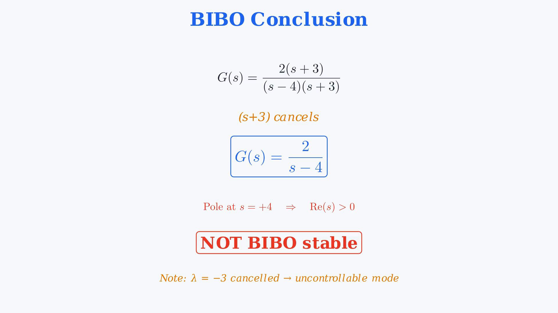
The state model and the cubic transfer function are separate problems. In the Routh figure, negative infinity records a one-sided limit; for every small positive epsilon the actual entry is finite.
The same factor appears in the numerator and denominator.
Cancel that common factor in the zero-state rational expression.
Reduced transfer function:
$\displaystyle G_{b}\left(s\right) =\frac{ 2}{s-4}$
The only remaining finite pole is:
$\displaystyle p = 4$
The positive pole lies in the open right half plane.
The input-output map is not BIBO stable.
Interpret the canceled internal mode.
The eigenvalue minus three is present in the state model but absent from the reduced transfer function.
Here that mode is unreachable from the input; the state equation and controllability rank verify the reason.
The minimal zero-state input-output map retains the dynamics that are both reachable and observable.
Narration transcript
Notice the factor s plus 3 appears in both numerator and denominator. It cancels. G of s simplifies to 2 divided by s minus 4. This transfer function has a single pole at s equals 4. The pole at positive 4 is in the right half plane. Conclusion: the system is NOT BIBO stable. Side note: the cancellation tells us something deeper. The eigenvalue negative 3 appeared in A but not in the transfer function. That mode is called an uncontrollable mode — the input b cannot reach it. The transfer function only sees the part of the dynamics that is both reachable from the input and observable at the output.
6. Keep the missing quadratic coefficient in the new denominator
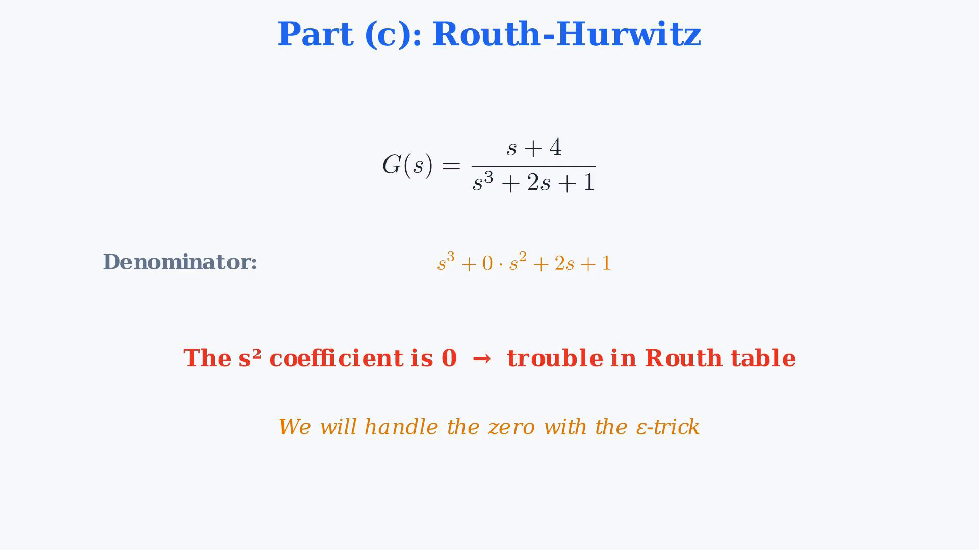
The state model and the cubic transfer function are separate problems. In the Routh figure, negative infinity records a one-sided limit; for every small positive epsilon the actual entry is finite.
Apply Routh to the separate function in part c.
New transfer function:
$\displaystyle G_{c}\left(s\right) =\frac{s+4}{s^{3}+2\cdot s+1}$
Its denominator is:
$\displaystyle P\left(s\right) = s^{3}+2\cdot s+1$
Keep the missing coefficient explicitly:
$\displaystyle P\left(s\right) = s^{3}+0\cdot s^{2}+2\cdot s+1$
The zero creates a first-column pivot problem.
Use the positive-infinitesimal procedure for this nonzero row.
Narration transcript
Part c: apply the Routh-Hurwitz criterion to a new transfer function. G of s equals s plus 4, divided by s cubed plus 2 s plus 1. The denominator is s cubed plus 2 s plus 1. Notice that the coefficient of s squared is zero. This is going to cause an unusual situation in the Routh table. Let us see how to handle it.
7. Resolve the zero pivot with a positive infinitesimal
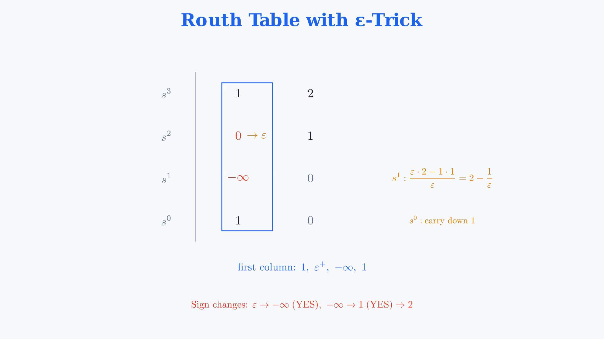
The state model and the cubic transfer function are separate problems. In the Routh figure, negative infinity records a one-sided limit; for every small positive epsilon the actual entry is finite.
Build the cubic Routh array in descending powers.
Cubic row:
$\displaystyle r_{3} = \left(1,2\right)$
Quadratic row before replacement:
$\displaystyle r_{2} = \left(0,1\right)$
The first pivot in this row is zero, but the entire row is not zero.
The ordinary next-row formula would divide by zero.
Replace the pivot by a positive epsilon and take its one-sided limit toward zero.
First-power entry with the perturbed pivot:
$\displaystyle c_{1} =\frac{\varepsilon \cdot 2-1\cdot 1}{\varepsilon }$
Simplify with the numerator grouped:
$\displaystyle c_{1} =\frac{2\cdot \varepsilon -1}{\varepsilon }= 2-\frac{1}{\varepsilon }$
This finite entry is negative for epsilon below one half and tends to negative infinity as epsilon tends to zero from above.
The constant row remains:
$\displaystyle r_{0} = \left(1,0\right)$
Finite first column:
$\displaystyle v = \left(1,\varepsilon ,2-\frac{1}{\varepsilon },1\right)$
Count sign changes for sufficiently small positive epsilon.
Positive one to positive epsilon adds no change.
Positive epsilon to the negative third entry adds one change.
The negative third entry to positive one adds a second change.
Right-half-plane root count:
$\displaystyle N_{\mathrm{RHP}} = 2$
Narration transcript
Build the Routh table. For a third-order polynomial, the first row is s cubed with coefficients 1 and 2 — the coefficients of s cubed and s. The second row is s squared with coefficients 0 and 1 — the coefficients of s squared and the constant. We have a zero in the first column of the s squared row. The standard Routh formula would divide by zero, which is undefined. The trick is to replace the zero with a small positive number epsilon, and take the limit as epsilon approaches zero. The s one row has one entry in the first column: the Routh formula gives epsilon times 2 minus 1 times 1, divided by epsilon. That is 2 epsilon minus 1, over epsilon, which equals 2 minus 1 over epsilon. As epsilon approaches zero from above, 1 over epsilon goes to plus infinity, so the whole expression goes to negative infinity. The s zero row simply carries down the constant, which is 1. So the first column reads: 1, epsilon, negative infinity, 1. Count the sign changes. From 1 to epsilon, both positive, no change. From epsilon to negative infinity, positive to negative, one sign change. From negative infinity to 1, negative to positive, another sign change. Total: 2 sign changes.
8. Count the two genuine right-half-plane poles
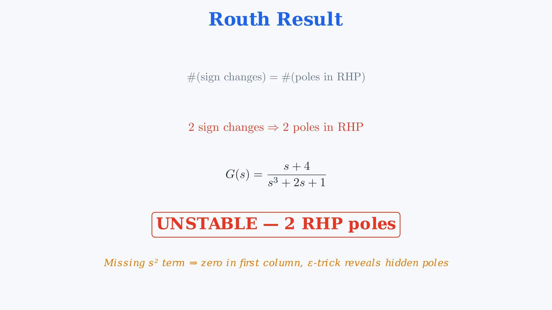
The state model and the cubic transfer function are separate problems. In the Routh figure, negative infinity records a one-sided limit; for every small positive epsilon the actual entry is finite.
The two sign changes imply two right-half-plane denominator roots.
They are uncanceled poles of:
$\displaystyle G_{c}\left(s\right) =\frac{s+4}{s^{3}+2\cdot s+1}$
This separate transfer function is unstable.
Do not omit a zero coefficient when constructing the array.
Resolving the zero pivot exposes the two right-half-plane roots; these are not canceled internal modes.
Narration transcript
By the Routh-Hurwitz criterion, 2 sign changes in the first column means 2 poles in the right half plane. So the transfer function G of s equals s plus 4 over s cubed plus 2 s plus 1 has 2 unstable poles. Conclusion: the system is not stable. Key lesson: a missing s squared term is not a special case you can ignore. The zero coefficient creates a zero in the Routh first column, and the epsilon trick reveals hidden right-half-plane poles.
9. Compare all three stability conclusions
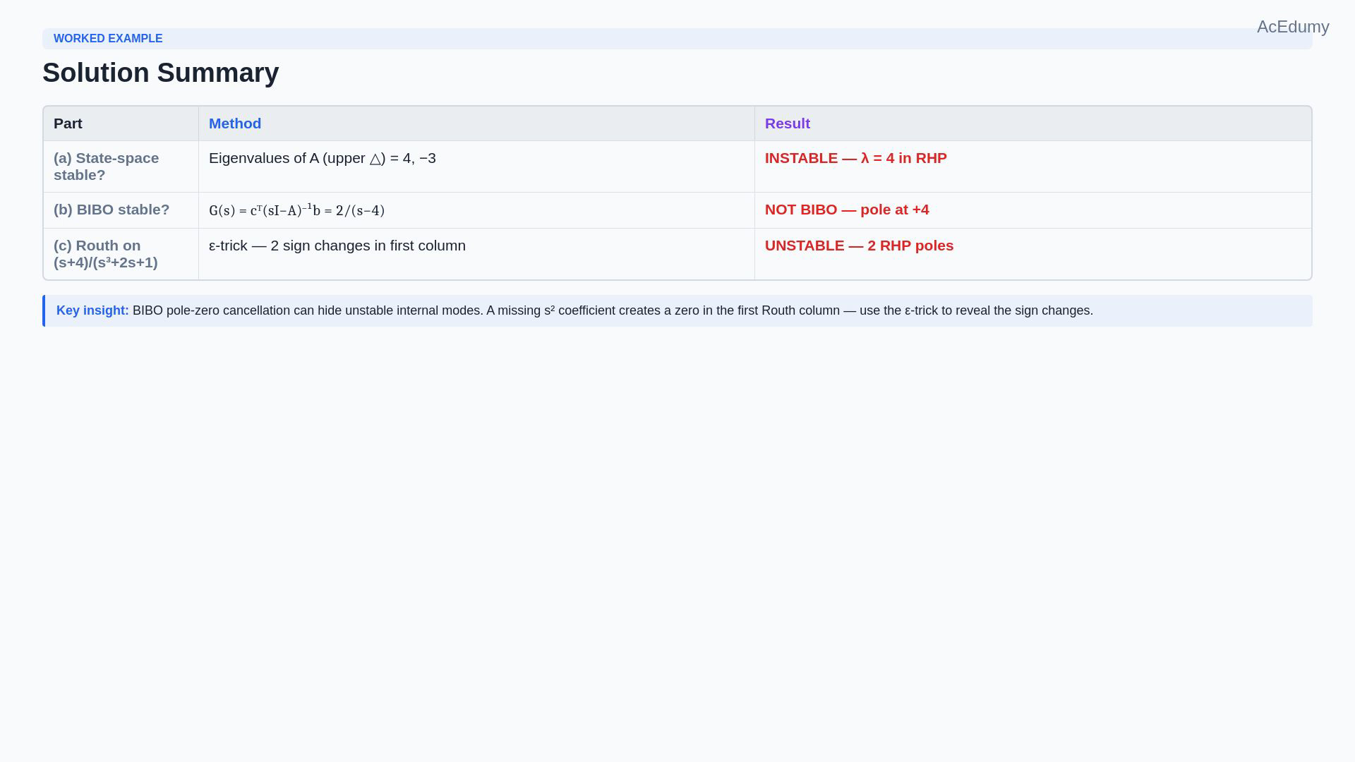
The state model and the cubic transfer function are separate problems. In the Routh figure, negative infinity records a one-sided limit; for every small positive epsilon the actual entry is finite.
Review the three questions.
Keep each stability test tied to its own model.
Part a uses internal eigenvalues.
State eigenvalues:
$\displaystyle \lambda _{1} = 4; \lambda _{2} = -3$
The positive eigenvalue makes the state model unstable.
Part b uses the zero-state BIBO map.
Reduced transfer function:
$\displaystyle G_{b}\left(s\right) =\frac{ 2}{s-4}$
The positive pole makes the map non-BIBO.
The canceled stable mode at minus three is unreachable from the input and remains part of the internal realization.
Part c uses the separate cubic with its zero quadratic coefficient.
The positive-infinitesimal Routh column has two sign changes and two right-half-plane poles.
All three requested tests give unstable outcomes, for the stated distinct reasons.
Narration transcript
Let us summarize. Three stability checks. Part a: internal stability from state space. A is upper triangular with eigenvalues 4 and negative 3. Eigenvalue 4 is in the right half plane, so the state space model is instable. Part b: BIBO stability. We derived the transfer function G equals 2 over s minus 4, with pole at positive 4. Not BIBO stable. The cancellation revealed an uncontrollable mode at negative 3. Part c: Routh-Hurwitz on a new third-order denominator with a zero s squared coefficient. The epsilon trick gave 2 sign changes in the first column, meaning 2 unstable poles. Three stability questions, three unstable answers.