Control Theory · From the Suspension State Model to Both Transfer Functions

#30 Choose position and velocity states, preserve the spring sign, and use the matrix resolvent for each input

Derive the voltage and road displacement maps from the same two-state suspension model.

Question

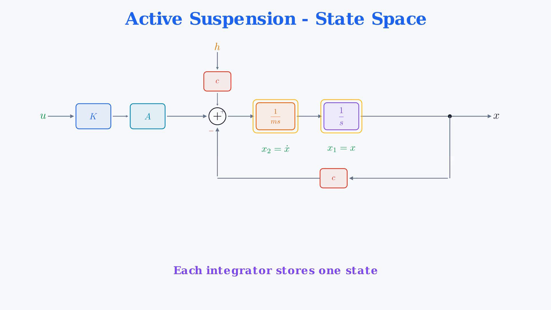
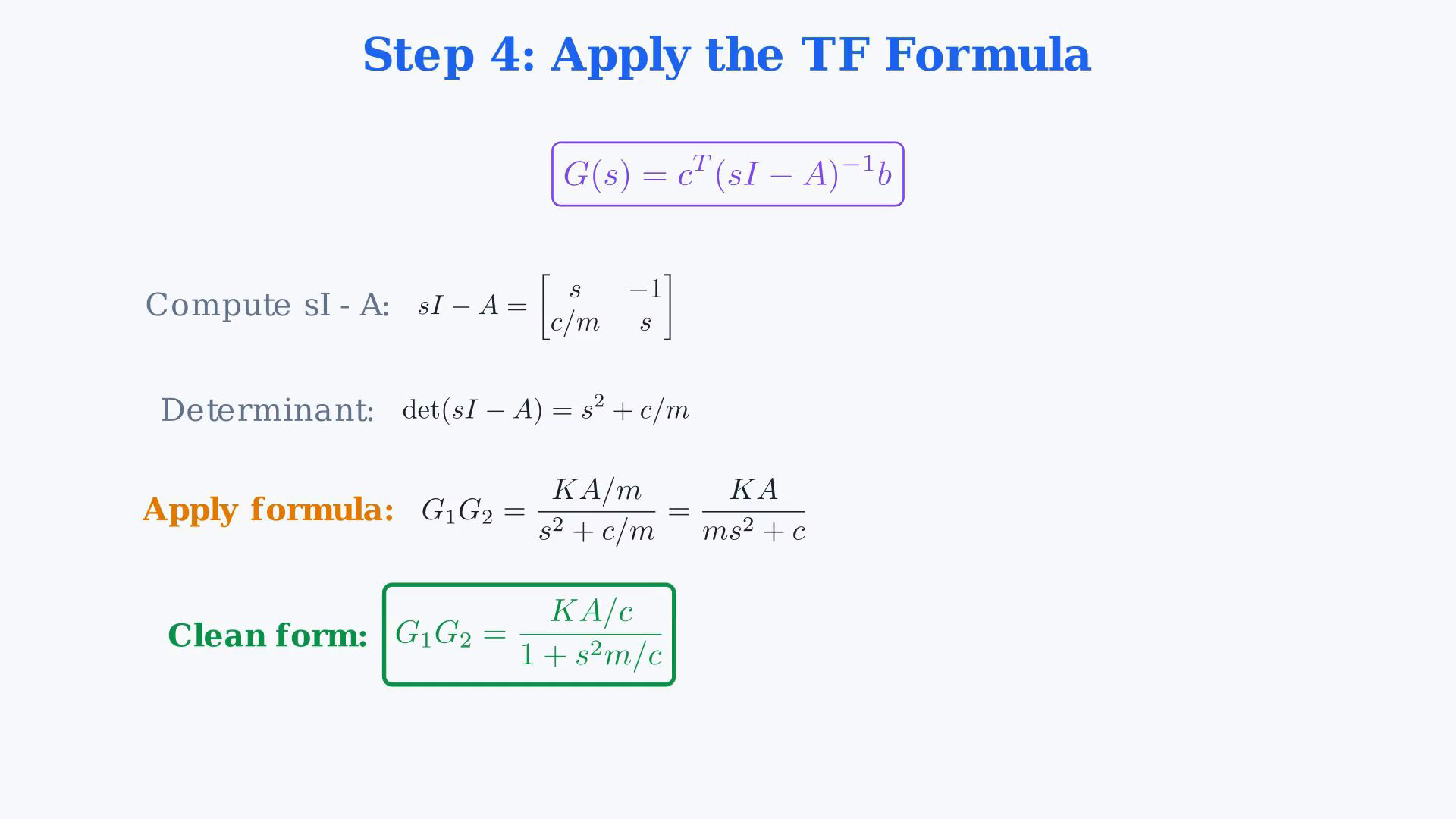
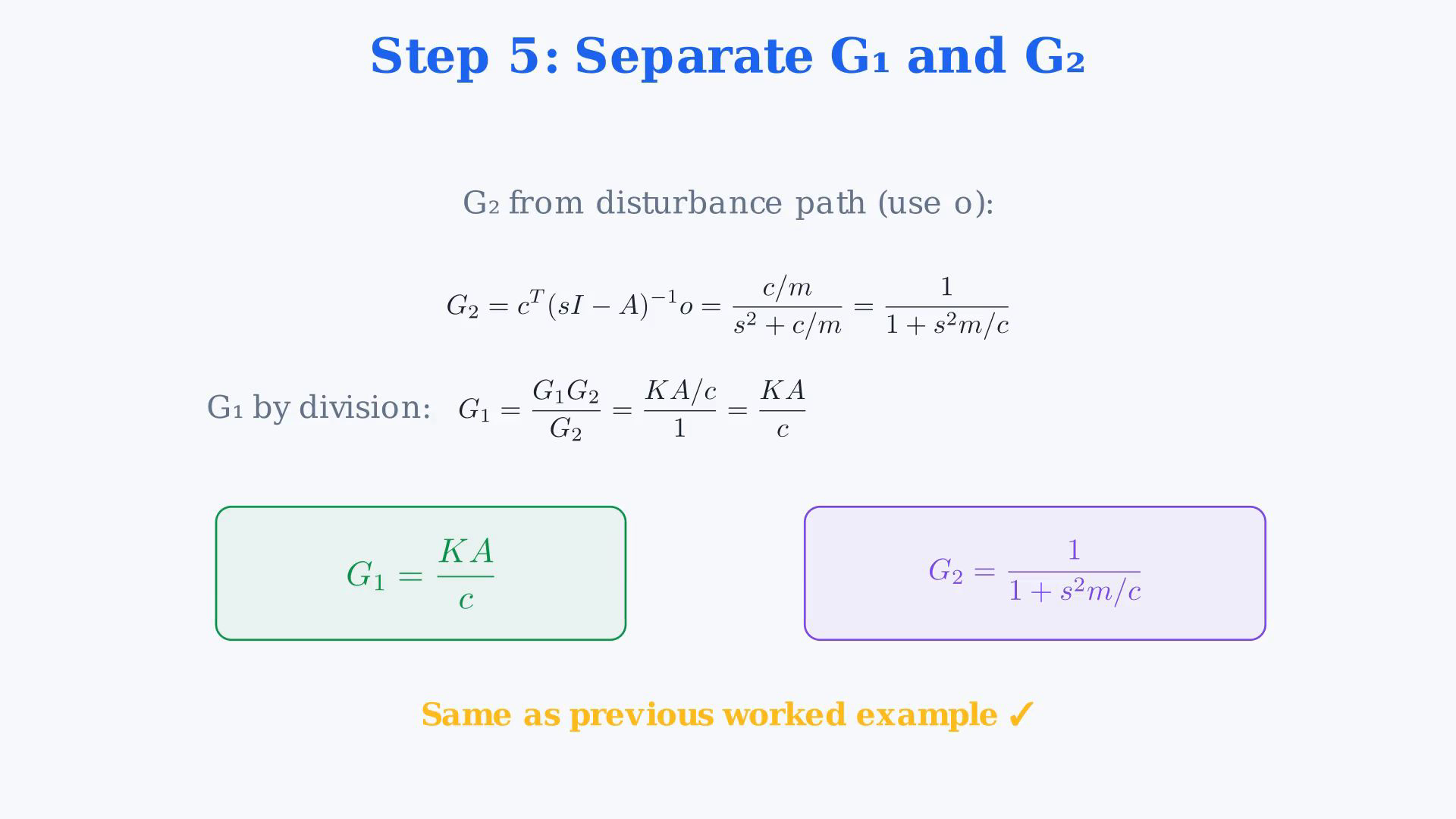
Existing final-video frame showing the correctly signed suspension model, state equations, system matrices or either input transfer calculation. — The spring stiffness c is distinct from the output row vector. The inverse applies to the entire matrix sI minus the system matrix. Follow the voltage and road input columns separately.

Consider the stated continuous-time linear undamped suspension model, with mass m>0, spring stiffness c>0, cylinder area A>0 and finite pressure-to-voltage coefficient K. Here c is a spring constant, not a damping coefficient. The variables are increments about a loaded static equilibrium: the static spring and actuator forces balance gravity, and their constant equilibrium terms have already been removed. The model is m x''=c(w-x)+KAu, with w=h the road displacement, u the actuator voltage and y=x the mass displacement. No additional damping or feedback controller is supplied. Positive spring stiffness alone does not establish asymptotic or BIBO stability. Use x1=x and x2=x' as states and write the state column as z=[x1,x2] transpose. The equations are x1'=x2 and x2'=-(c/m)x1+(KA/m)u+(c/m)w. In the grouped form, c/m multiplies the entire difference (w-x1). The source's spoken 'c over m times w minus state one' is read with the preceding explicit 'quantity w minus state one', the parenthesized equation on the actual frame and the subsequent explicit negative coefficient -c/m. It does not mean (c/m)w-x1. The integrator driven by force divided by mass stores velocity; the next integrator stores position. The video uses A for both the cylinder area and, in matrix context, the state matrix. It also uses c for spring stiffness and c transpose for the output row. To distinguish these objects in the notebook, call the state matrix A_sys and the output row C_y. These are explicit notation changes only: A_sys is the video's system matrix A, and C_y is its c transpose. The area A and stiffness c retain their physical meanings. The disturbance column is the letter o, not the scalar zero. Thus z'=A_sys z+b u+o w, with A_sys rows [0,1] and [-c/m,0], b=[0,KA/m] transpose, o=[0,c/m] transpose and C_y=[1,0]. The output is y=C_y z. Both direct input-to-output terms are zero; neither u nor w appears directly in the output equation. For zero initial states, compute each external input map with the same matrix resolvent R(s)=(sI-A_sys) inverse. Here sI-A_sys has rows [s,-1] and [c/m,s]; its determinant is s²+c/m. Its inverse is 1/(s²+c/m) times the matrix with rows [s,1] and [-c/m,s]. The entire matrix is inverted; do not read this as sI minus A_sys inverse. The multiplication order C_y R b or C_y R o matters because matrix products do not generally commute. Use the inverse only at values of s where its determinant is nonzero, with the usual transfer-function continuation as a rational function. A nonzero determinant at one value of s is not a stability proof. With the other input set to zero, the voltage-to-position map is G_u=C_y R b=(KA/m)/(s²+c/m)=KA/(ms²+c)=(KA/c)/(1+s²m/c). The road-to-position map is G_w=C_y R o=(c/m)/(s²+c/m)=c/(ms²+c)=1/(1+s²m/c). For both inputs present, Y=G_u U+G_w W in the zero state. The source labels G2=G_w and G1G2=G_u, hence G1=G_u/G_w=KA/c wherever that ratio is evaluated. Since c>0, this simplification is a valid rational identity. G1 by itself is the voltage-to-equivalent-displacement gain of the factorization; it is not the complete voltage-to-position transfer. G2 is dimensionless, while G1 and G_u carry length per voltage. The coefficient c/m has units of inverse seconds squared. Verify independently from the original force balance: with zero initial conditions its Laplace transform is (ms²+c)Y=KAU+cW. This checks both input numerators and the restoring-force minus sign. The final G1 and G2 agree with the correct final formulas shown in the preceding worked example; agreement of these final formulas does not establish the validity of every intermediate block-diagram manipulation in another presentation. The state equations also describe nonzero initial position and velocity, but the transfer formula alone does not include their response. In general Y=C_y R b U+C_y R o W+C_y R z(0). With no input, x(t)=x(0)cos(omega0 t)+x'(0)sin(omega0 t)/omega0, where omega0=sqrt(c/m). The two poles are on the imaginary axis at plus and minus j omega0. Free oscillations persist rather than decay, and a bounded road input at that natural frequency can cause an unbounded resonant response. Thus this ideal undamped model is not asymptotically stable or BIBO stable. The task is to preserve the given physical model through the state-space calculation, not to infer damping or a controller from its name.

Written solution and narration transcript(shows the full solution)

Below are all the lines written in the notebook together with the full narration transcript.

1. Recall the physical model
The spring stiffness c is distinct from the output row vector. The inverse applies to the entire matrix sI minus the system matrix. Follow the voltage and road input columns separately.
Return to the active suspension model.
The force balance and two integrators describe the same physical system.
The earlier final factorization contains G₁ and G₂.
Derive both input maps using position and velocity states.
Zero-state voltage map:
$\displaystyle G_{u}\left(s\right) = C_{y}\cdot \left(s\cdot I-A_{\mathrm{sys}}\right)^{-1}\cdot b$
Use A_sys for the state matrix and C_y for the output row; A is area and c is spring stiffness.
Narration transcript
Welcome back to the active suspension system. In an earlier video we modeled the system from physics and built its block diagram. In the next video we simplified that block diagram and found the transfer functions G1 and G2 by series, junction move, and feedback rules. Today we will reach the same answer using a completely different method: state space. We will write the state equations, build the A, b, c matrices, then apply the matrix formula G of s equals c transpose times s I minus A inverse times b. Same physical system, same answer, new technique.
2. Choose position and velocity states
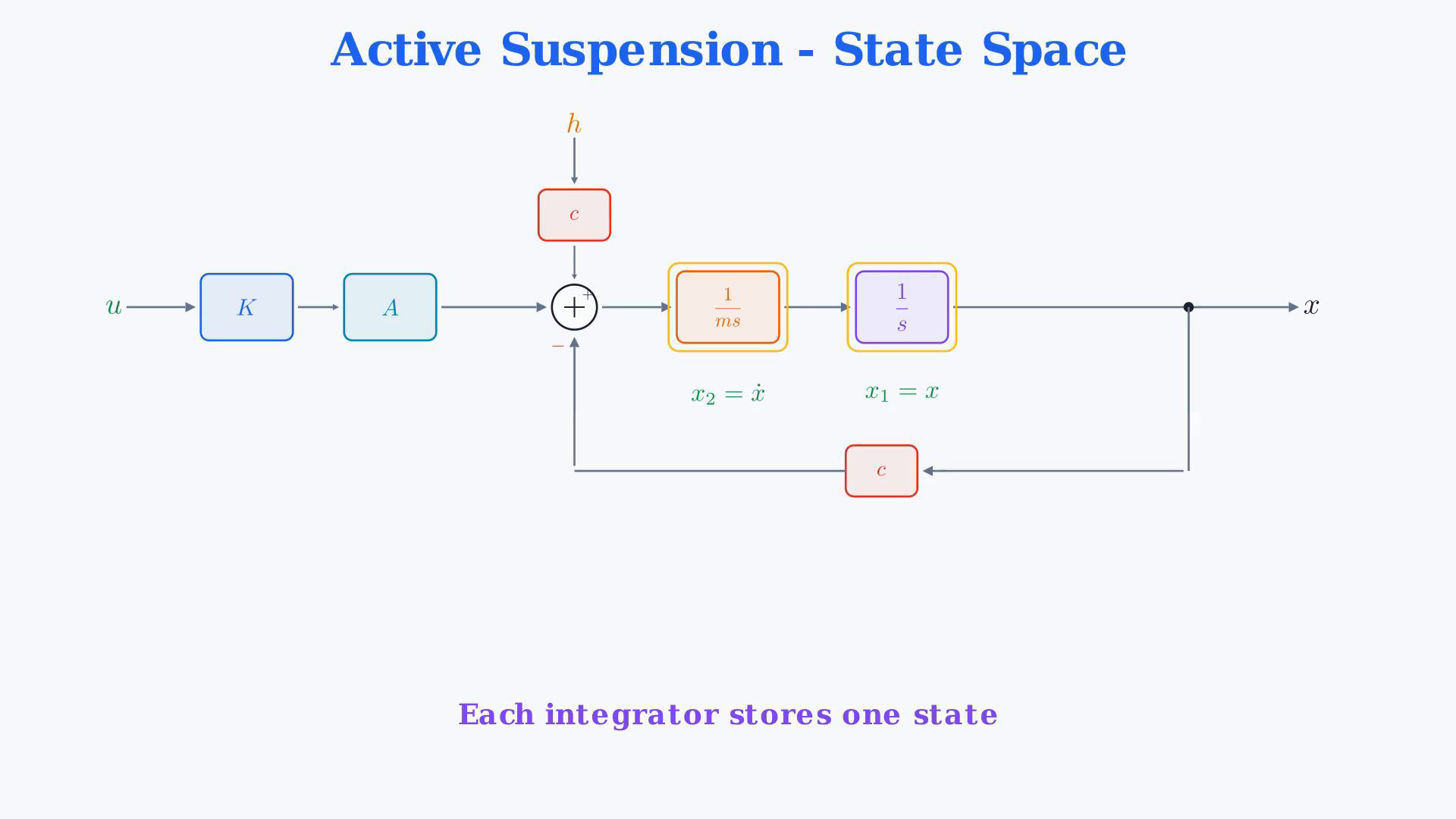
The spring stiffness c is distinct from the output row vector. The inverse applies to the entire matrix sI minus the system matrix. Follow the voltage and road input columns separately.
Choose the states.
There are two integrators in series.
Each integrator stores one state.
Label their outputs from position back toward velocity.
Position state:
$\displaystyle x_{1} = x$
Velocity state:
$\displaystyle x_{2} = x'$
Together these two states describe the mass motion.
The voltage u is the actuator input.
Road displacement:
$\displaystyle w = h$
Output:
$\displaystyle y = x_{1}$
Narration transcript
Step one: choose the states. Looking at the block diagram, we have two integrators in series. Each integrator stores one state. We name the integrator outputs from right to left. The output of the rightmost integrator is x, the position. The output of the middle integrator is the derivative of x, the velocity. So we set state one equals x, and state two equals x dot. The input is u, the voltage. The disturbance is w, equal to h, the road bumpiness. The output is y, equal to x, which is state one.
3. Write both state equations
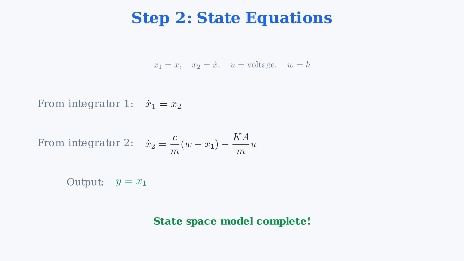
The spring stiffness c is distinct from the output row vector. The inverse applies to the entire matrix sI minus the system matrix. Follow the voltage and road input columns separately.
Write the two state equations.
The position integrator receives the velocity.
First state equation:
$\displaystyle x_{1}' = x_{2}$
This equation records the position derivative.
Force divided by mass drives the velocity integrator.
Total incremental force:
$\displaystyle F = c\cdot \left(w-x_{1}\right)+K\cdot A\cdot u$
Divide the complete force expression by the positive mass.
Second state equation:
$\displaystyle x_{2}' = \left(\frac{c}{m}\right)\cdot \left(w-x_{1}\right)+\left(K\cdot \frac{A}{m}\right)\cdot u$
Output equation:
$\displaystyle y = x_{1}$
The two state equations and output relation complete the model.
Narration transcript
Step two: write the state equations. From the block diagram, the first integrator turns x dot into x. So the derivative of state one equals state two. That is the first equation. The second integrator is fed by the total force divided by mass m. The total force entering the integrator is c times the quantity w minus state one, plus K times A times u. Divide everything by m. So the derivative of state two equals c over m times w minus state one, plus K A over m times u. The output equation is simple: y equals state one. We have a complete state space model.
4. Separate the system and input matrices
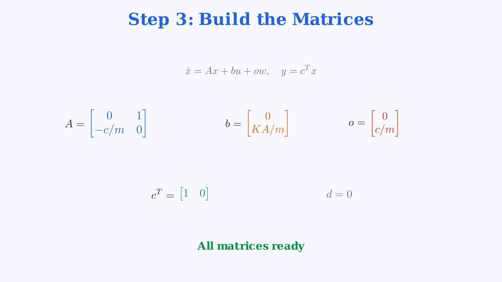
The spring stiffness c is distinct from the output row vector. The inverse applies to the entire matrix sI minus the system matrix. Follow the voltage and road input columns separately.
Extract the system matrix and both input columns.
Use the state column z with position first and velocity second.
State form:
$\displaystyle z' = A_{\mathrm{sys}}\cdot z+b\cdot u+o\cdot w$
First row of A_sys: zero, one. First entries of b and o: zero.
Second row of A_sys: minus c/m, zero; the spring force restores position.
Voltage column, second entry:
$\displaystyle b_{2} =\frac{K\cdot A}{m}$
Road column, second entry:
$\displaystyle o_{2} =\frac{ c}{m}$
C_y is the row one, zero; both direct input terms are zero.
Narration transcript
Step three: extract the matrices. Rewrite the two state equations in matrix form. The derivative of x equals A times x plus b times u plus o times w. From state one equation: derivative is just state two, so the first row of A is zero one, and the first elements of b and o are zero. From state two equation: state one appears with coefficient minus c over m, state two does not appear, so the second row of A is minus c over m, zero. The coefficient of u is K A over m, so the second element of b is K A over m. The coefficient of w is c over m, so the second element of o is c over m. For the output, y equals state one, so c transpose is one zero, and d is zero.
5. Compute the voltage-to-position transfer
The spring stiffness c is distinct from the output row vector. The inverse applies to the entire matrix sI minus the system matrix. Follow the voltage and road input columns separately.
Apply the zero-state transfer formula.
Voltage-to-position map:
$\displaystyle G_{u}\left(s\right) = C_{y}\cdot \left(s\cdot I-A_{\mathrm{sys}}\right)^{-1}\cdot b$
Form the complete matrix sI minus A_sys.
The diagonal entries of sI are s; its other entries are zero.
The resulting rows are s, minus one; and c/m, s.
Determinant:
$\displaystyle D\left(s\right) = s^{2}+\frac{c}{m}$
The inverse has rows s, one; and minus c/m, s, all divided by D(s).
Multiply the output row, then this inverse, then the voltage column.
Voltage map:
$\displaystyle G_{u}\left(s\right) =\frac{\frac{K\cdot A}{m}}{s^{2}+\frac{c}{m}}$
Clear the mass fraction:
$\displaystyle G_{u}\left(s\right) =\frac{K\cdot A}{m\cdot s^{2}+c}$
Factor the stiffness:
$\displaystyle G_{u}\left(s\right) =\frac{\frac{K\cdot A}{c}}{1+s^{2}\cdot \frac{m}{c}}$
Connection to the factorization:
$\displaystyle G_{u} = G_{1}\cdot G_{2}$
Narration transcript
Step four: apply the transfer function formula. We use G of s equals c transpose times s I minus A inverse times b for the transfer function from u to y. First compute s I minus A. The matrix s I is s on the diagonal, zero elsewhere. Subtract A: the result is s, minus one in the first row, c over m, s in the second row. Compute its determinant: s times s minus minus one times c over m, equals s squared plus c over m. So the inverse is one over s squared plus c over m, times the matrix s, one, minus c over m, s. Now multiply: c transpose, then the inverse, then b. The result is K A over m, divided by s squared plus c over m. Multiply numerator and denominator by m to clean up: K A divided by m s squared plus c. Factor c from the denominator: K A over c, divided by one plus s squared m over c. This is G one times G two.
6. Compute the road-to-position transfer
The spring stiffness c is distinct from the output row vector. The inverse applies to the entire matrix sI minus the system matrix. Follow the voltage and road input columns separately.
Separate the road response and the voltage gain.
G₂ is the road-to-position map, with voltage set to zero.
Use the road column:
$\displaystyle G_{2}\left(s\right) = C_{y}\cdot \left(s\cdot I-A_{\mathrm{sys}}\right)^{-1}\cdot o$
The column o has entries zero and c/m; o is a letter, not zero.
Road map:
$\displaystyle G_{2}\left(s\right) =\frac{\frac{c}{m}}{s^{2}+\frac{c}{m}}$
Clear the mass fraction:
$\displaystyle G_{2}\left(s\right) =\frac{ c}{m\cdot s^{2}+c}$
Factor the stiffness:
$\displaystyle G_{2}\left(s\right) =\frac{ 1}{1+s^{2}\cdot \frac{m}{c}}$
This dimensionless map takes road displacement to mass displacement.
Divide the complete maps:
$\displaystyle G_{1} =\frac{ G_{u}}{G_{2} }=\frac{K\cdot A}{c}$
Both inputs together:
$\displaystyle Y = G_{1}\cdot G_{2}\cdot U+G_{2}\cdot W$
These are the correct final formulas of the earlier factorization.
The original force balance independently verifies both input maps.
Narration transcript
Step five: separate G one and G two and verify. We need G two by itself, the transfer function from disturbance w to output y. Apply the same formula but with o instead of b: G two equals c transpose times s I minus A inverse times o. The o vector is zero, c over m. Multiply: the result is c over m divided by s squared plus c over m. Clean up: c divided by m s squared plus c. Factor c again: one divided by one plus s squared m over c. So G two equals one over one plus s squared m over c. Now G one comes from dividing G one G two by G two: K A over c divided by one, equals K A over c. The result: G one equals K A over c, and G two equals one over one plus s squared m over c. These match exactly the answers we got in the previous video using block diagram simplification. Two methods, one truth.
7. Check both resulting input maps
The spring stiffness c is distinct from the output row vector. The inverse applies to the entire matrix sI minus the system matrix. Follow the voltage and road input columns separately.
Review the state-space derivation.
Start with the same incremental, undamped suspension model.
Use its position and velocity states.
Choose the outputs of the two integrators.
Derive the state equations from the signed force balance.
Separate the state matrix, voltage column, road column and output row.
Voltage map:
$\displaystyle G_{1}\cdot G_{2} = C_{y}\cdot \left(s\cdot I-A_{\mathrm{sys}}\right)^{-1}\cdot b$
Use o for the road map, then divide to find the voltage gain G₁.
Final factorization:
$\displaystyle G_{1} =\frac{K\cdot A}{c}; G_{2} =\frac{ 1}{1+s^{2}\cdot \frac{m}{c}}$
The zero-state maps agree with the original physical equation.
Initial-state response and undamped resonance require separate attention.
Narration transcript
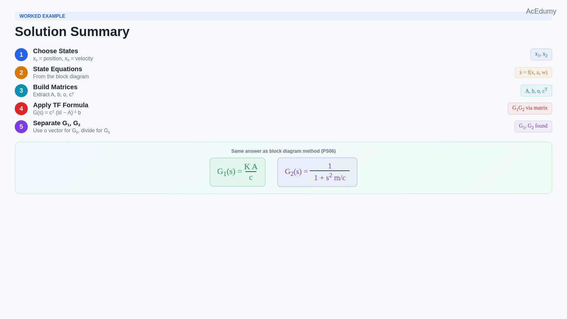
Let us recap. We took the active suspension system, the same one we modeled in our first worked example and simplified in our previous worked example. This time we used state space. Step one: we chose the integrator outputs as states, position and velocity. Step two: we wrote the state equations from the block diagram. Step three: we extracted the A, b, o, c matrices. Step four: we computed s I minus A inverse, then applied the c transpose s I minus A inverse b formula to get G one G two. Step five: we used the o vector to get G two alone, then divided to get G one. Final answer: G one equals K A over c, and G two equals one over one plus s squared m over c. Same as before, by a different method. Two paths, same destination.