Control Theory · Steady-State Error

#22 Predict stable unity-feedback tracking with system type and position, velocity and acceleration error constants

Separate the tracking-error constants and check the stability conditions before applying the final-value theorem.

Question

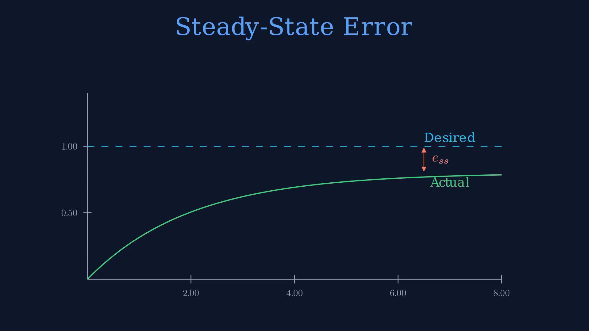
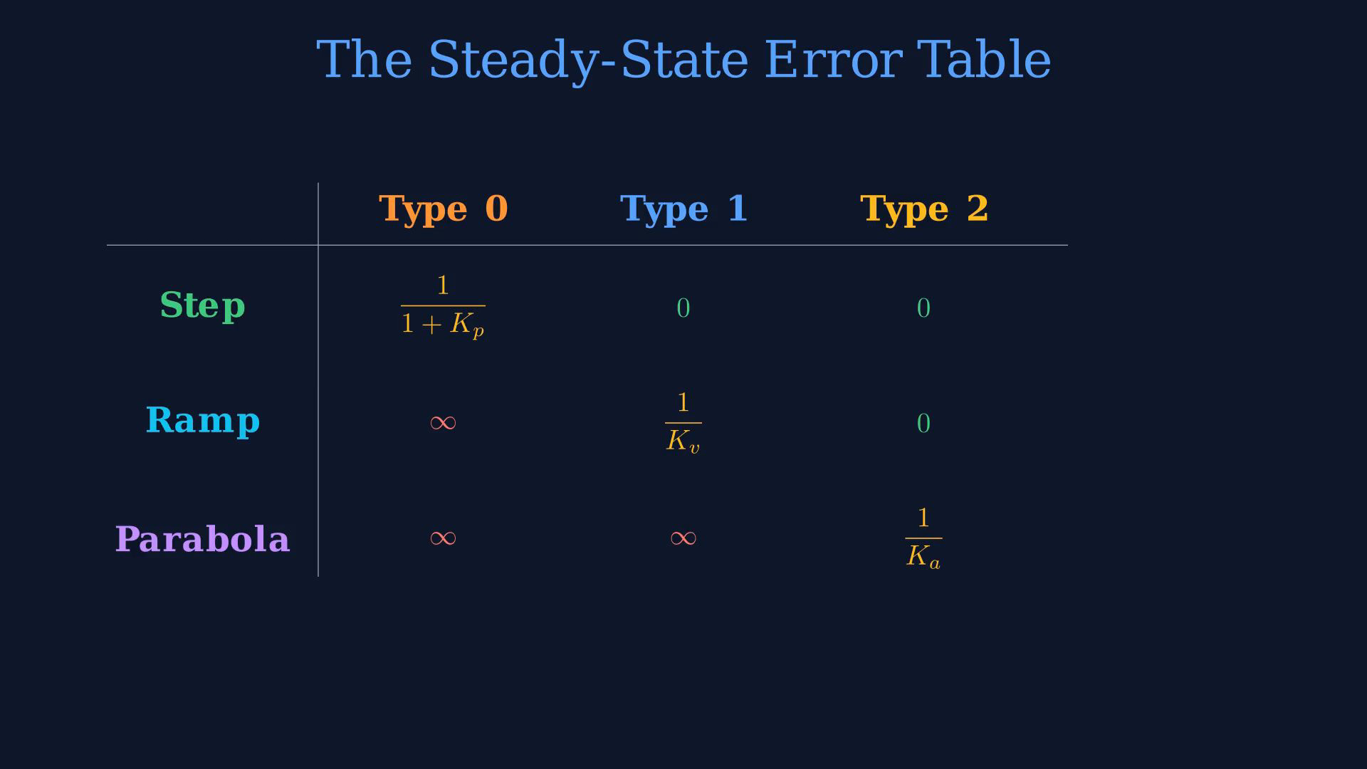
Existing lesson frame showing a tracking error, negative unity-feedback relation, system-type card, error table or worked example. — Use the stability and normalization conditions in the problem statement. Step arrows mark asymptotic gaps. System-type cards classify origin poles only. Ramp and summary sections use the existing error table as their reference; its infinity entries describe unbounded errors, not finite limits.

Work with a well-posed continuous-time, scalar SISO LTI negative unity-feedback system in the zero state. Use real rational proper transfer functions, and check internal stability rather than relying on a cancellation that hides an unstable mode. The forward transfer is G(s), the reference transform is R(s), and the output is Y(s). Define e(t)=r(t)-y(t), E(s)=R(s)-Y(s), Y(s)=G(s)E(s), so E(s)=R(s)/(1+G(s)). These equations depend on the feedback sign and unity sensor gain. Nonunity sensing, disturbances, saturation, nonlinear dynamics and nonzero initial states require their own equations. Negative feedback by itself does not guarantee stability. The finite final-value formula is e_ss=lim as s approaches zero of s E(s), provided all poles of s E(s) are strictly in the left half-plane for these rational causal signals. Equivalently E can have at most a simple origin pole, with all other poles strictly left. A right-half-plane or nonzero imaginary-axis pole invalidates the finite final-value conclusion even if formal substitution gives a number. The infinity entries in the table denote unbounded long-time error; they are not a use of the finite final-value theorem for a higher-order origin pole. Check stability first, then the behavior of the particular error transform. System type is the net number of poles at the origin in the reduced open-loop G(s), after common factors are cancelled. A denominator symbol s alone is not sufficient if the numerator cancels it. The displayed K/(s+a), K/[s(s+a)] and K/[s squared(s+a)] cards classify Types zero, one and two only for nonzero K and nonzero a. These cards do not assert stable closed-loop tracking. In particular the Type-two card with positive a and K gives the closed-loop characteristic polynomial s cubed+a s squared+K, whose Routh first column is 1, a, -K/a, K and has two sign changes: two right-half-plane poles. Adding integrators can destabilize a feedback loop. Internal stability and hidden cancellations must be assessed independently of the external type count. Use normalized causal references: a unit step is H(t) with transform 1/s; a unit ramp is t H(t) with transform 1/s squared; the unit parabola here is t squared H(t)/2 with transform 1/s cubed. If instead the reference is t squared, the parabolic error is twice the tabulated value. Scaling any reference by A scales its error by A. Define Kp=lim G(s), Kv=lim s G(s), and Ka=lim s squared G(s), with s tending to zero along the positive real axis. Position, velocity and acceleration are conventional names for these error constants; the signal need not be a mechanical position. Use the usual positive finite leading low-frequency gain for the positive infinity and lag-behind interpretations. Negative gain can give an error of the opposite sign or an output above the reference, and arbitrary signed systems do not inherit the figure's positive ordering. For stable negative unity feedback under these assumptions, Type zero has unit-step error 1/(1+Kp), unbounded ramp error, and unbounded parabolic error. Type one has zero step error, unit-ramp error 1/Kv, and unbounded parabolic error. Type two has zero step and ramp errors and unit-parabola error 1/Ka. Stable Type three or higher has zero errors for these three references. A finite nonzero leading error constant is understood at the system's own type order. Higher type improves the asymptotic classification only with stability retained; it cannot make an already-zero error strictly smaller and cannot guarantee transient speed or overshoot. Perfect tracking in the narration means the error tends to zero as time tends to infinity, not that it is identically zero during the transient. A constant ramp position offset means the output eventually has the same slope as the reference. Finite tracking error does not itself imply rejection of every disturbance. The intro and step plots illustrate separate positive-gain examples. The Type-zero curve approaches 0.8, so its limiting unit-step error is 0.2. The drawn arrows denote the asymptotic reference-to-limit gap, not the exact vertical distance to the finite-time curve at the arrow's horizontal location. The plotted responses are illustrative examples, not a claim that the type cards or the worked example have those identical transients. The original ramp illustration uses separate Type-zero, one and two curves; the error table supplies an unambiguous reference for this section. For the worked example G(s)=10(s+2)/[s(s+5)], the numerator is nonzero at zero, so there is one net integrator. The closed-loop denominator is s squared+15s+20, with roots (-15 plus or minus square root 145)/2, both negative; the relevant tracking limits therefore apply. Kp is positive infinity because the integrator remains in G. Kv=lim 10(s+2)/(s+5)=4, and Ka=0. The unit-step error tends to zero, the unit-ramp error tends to 1/4=0.25, and the unit-parabola error is unbounded. The source narration briefly says to cancel s in the Kp calculation, then explicitly retracts that result with 'Wait' and states that Kp is infinite, before correctly computing Kv as four. Preserve this correction as part of the example: the finite number four belongs to Kv and must never be reported as Kp. It is multiplication of G by s in the velocity-constant limit that cancels the origin factor. The displayed example card gives the corrected constants and errors. The root-locus method in the next lesson concerns how the closed-loop poles vary with gain.

Written solution and narration transcript(shows the full solution)

Below are all the lines written in the notebook together with the full narration transcript.

1. Define the tracking error
Use the stability and normalization conditions in the problem statement. Step arrows mark asymptotic gaps. System-type cards classify origin poles only. Ramp and summary sections use the existing error table as their reference; its infinity entries describe unbounded errors, not finite limits.
Recall transient speed and oscillation.
Ask whether the output approaches the requested value.
Tracking error:
$\displaystyle e\left(t\right) = r\left(t\right)-y\left(t\right)$
Predict the asymptotic error only after checking stability and the relevant limits.
Narration transcript
In the previous lessons, we focused on how fast a system responds and how much it oscillates. But there is another critical question: does the output actually reach the desired value? The difference between the desired and actual output in steady state is called the steady state error. Today we learn how to predict this error without simulating the system.
2. Use negative unity feedback
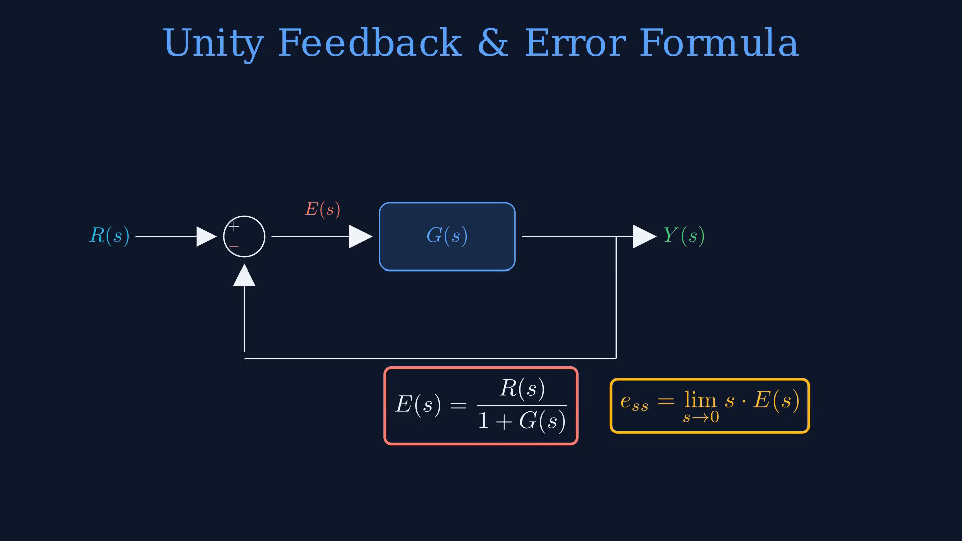
Use the stability and normalization conditions in the problem statement. Step arrows mark asymptotic gaps. System-type cards classify origin poles only. Ramp and summary sections use the existing error table as their reference; its infinity entries describe unbounded errors, not finite limits.
Use a well-posed negative unity-feedback interconnection.
Let R and Y be the zero-state input and output transforms, with forward transfer G.
Error transform:
$\displaystyle E\left(s\right) = R\left(s\right)-Y\left(s\right)$
Negative unity feedback:
$\displaystyle E\left(s\right) =\frac{ R\left(s\right)}{1+G\left(s\right)}$
When the final-value conditions hold, the steady-state error is the limit of s times E(s) as s tends to zero.
Narration transcript
Consider a unity feedback system. The input is R of s, the output is Y of s, and the forward path transfer function is G of s. The error signal is E of s equals R of s minus Y of s. Using the closed loop relationship, we can write E of s equals R of s divided by one plus G of s. The steady state error is found using the final value theorem: e steady state equals the limit as s approaches zero of s times E of s.
3. Count the net integrators
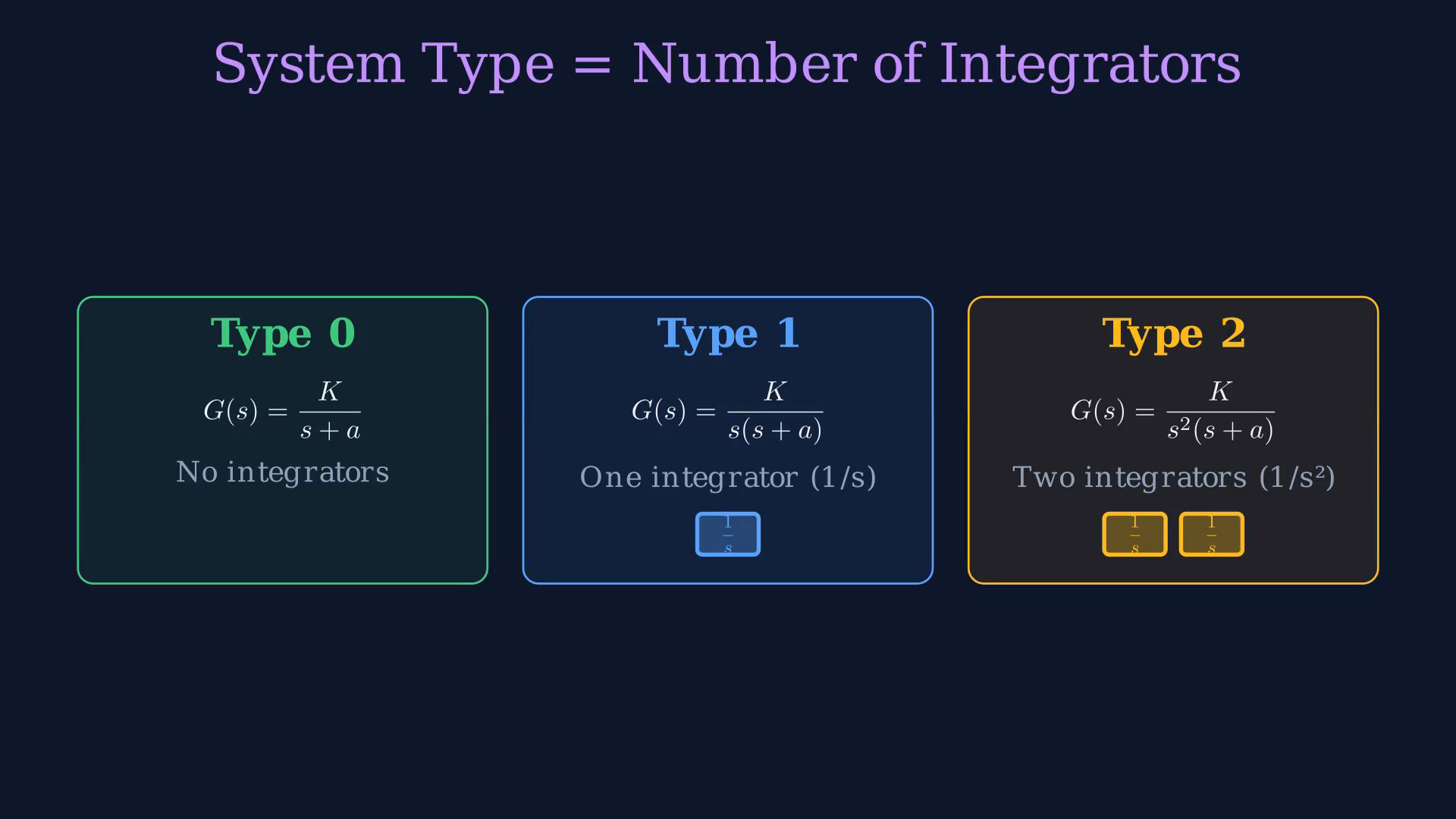
Use the stability and normalization conditions in the problem statement. Step arrows mark asymptotic gaps. System-type cards classify origin poles only. Ramp and summary sections use the existing error table as their reference; its infinity entries describe unbounded errors, not finite limits.
Count the poles at the origin in the reduced open-loop transfer G.
Type zero has no net integrators.
Type one has one uncancelled pole at the origin.
Type two has two net integrators.
Combine system type with closed-loop stability to predict asymptotic tracking.
Higher type can give zero asymptotic error for higher-degree polynomial inputs; it does not ensure stability or exact tracking at every time.
Narration transcript
The system type is the number of pure integrators in the open loop transfer function G of s. A Type zero system has no integrators. A Type one system has one integrator, meaning one s in the denominator. A Type two system has two integrators. The system type determines which inputs the system can track with zero error. Higher type means the system can track more complex inputs perfectly.
4. Track a unit step
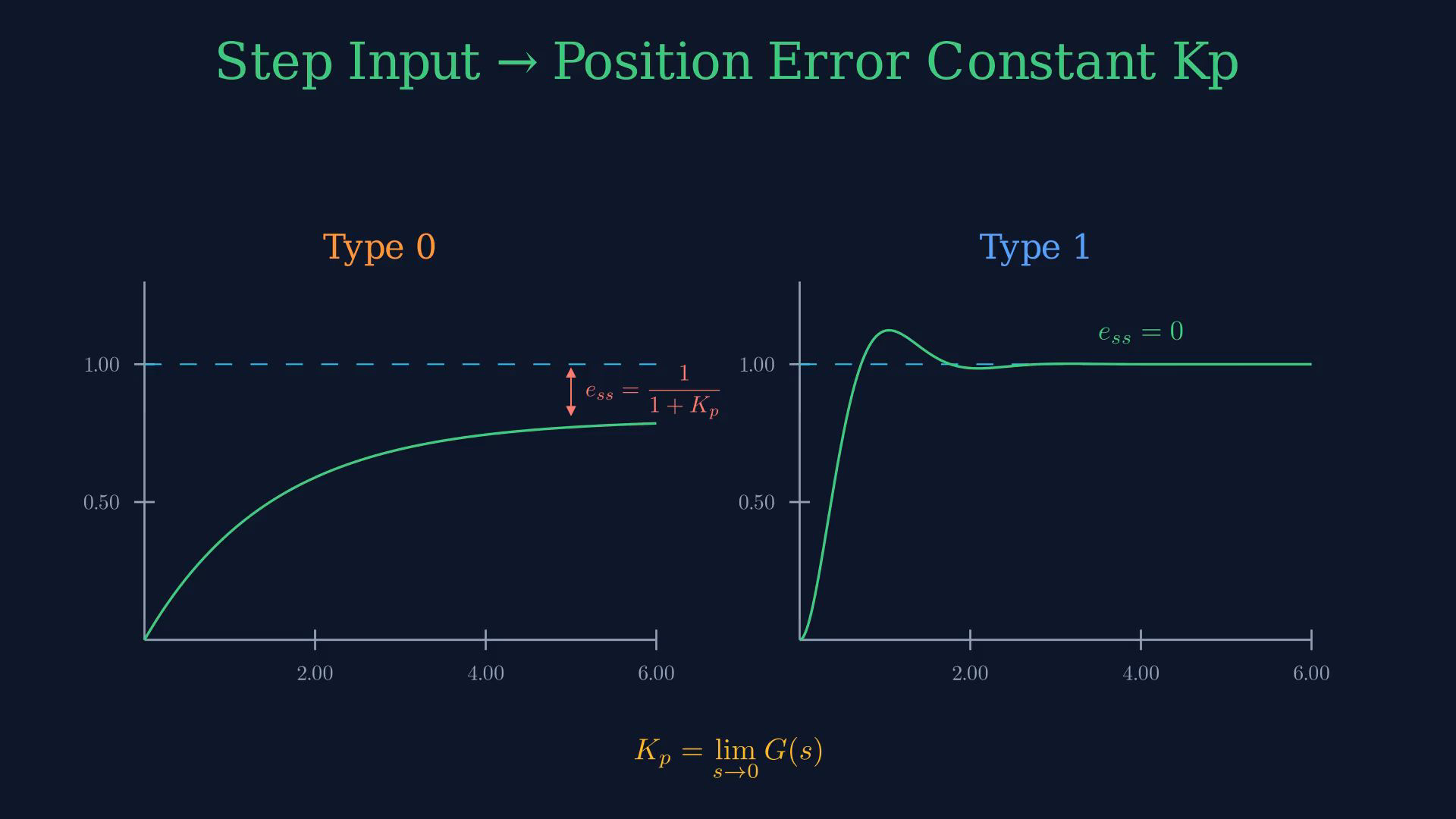
Use the stability and normalization conditions in the problem statement. Step arrows mark asymptotic gaps. System-type cards classify origin poles only. Ramp and summary sections use the existing error table as their reference; its infinity entries describe unbounded errors, not finite limits.
Unit-step transform:
$\displaystyle R\left(s\right) =\frac{ 1}{s}$
Qualified unit-step error:
$\displaystyle e_{\mathrm{ss}} =\frac{ 1}{1+K_{p}}$
The position constant Kₚ is the limit of G(s) as s tends to zero.
A finite Type-zero position constant gives a finite nonzero step error when the closed loop is stable.
A stable Type-one or higher loop has zero asymptotic step error.
The plotted Type-zero example has positive DC gain and approaches a value below one; the arrow indicates the asymptotic gap.
Narration transcript
For a unit step input, R of s equals one over s. The steady state error becomes one divided by one plus K p, where K p is the position error constant. K p equals the limit as s approaches zero of G of s. For a Type zero system, K p is finite, so there is a nonzero steady state error. For Type one or higher, K p is infinite, and the error is zero. Watch the step response: Type zero settles to a value less than one.
5. Track a unit ramp
Use the stability and normalization conditions in the problem statement. Step arrows mark asymptotic gaps. System-type cards classify origin poles only. Ramp and summary sections use the existing error table as their reference; its infinity entries describe unbounded errors, not finite limits.
Unit-ramp transform:
$\displaystyle R\left(s\right) = 1/s²$
Qualified unit-ramp error:
$\displaystyle e_{\mathrm{ss}} =\frac{ 1}{K_{v}}$
The velocity constant Kᵥ is the limit of s times G(s) as s tends to zero.
Type-zero ramp error grows without bound under the stated stable positive-gain assumptions.
The illustrated Type-zero output falls increasingly behind the ramp.
For stable Type one, the output approaches the same slope with a constant position offset.
For stable Type two, the ramp error tends to zero after the transient.
Narration transcript
For a unit ramp input, R of s equals one over s squared. The steady state error becomes one over K v, where K v is the velocity error constant. K v equals the limit as s approaches zero of s times G of s. A Type zero system has K v equals zero, so the ramp error is infinite. The output falls further and further behind the ramp. A Type one system has finite K v, giving a constant position offset. A Type two system tracks the ramp perfectly with zero error.
6. Track a unit parabola
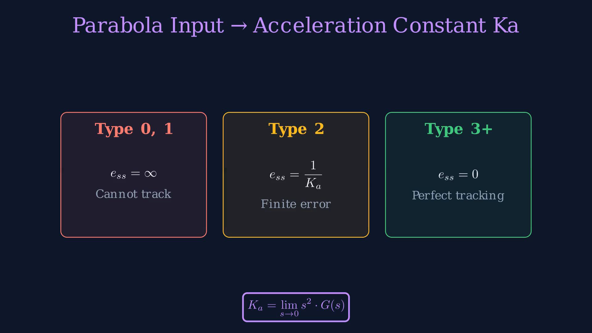
Use the stability and normalization conditions in the problem statement. Step arrows mark asymptotic gaps. System-type cards classify origin poles only. Ramp and summary sections use the existing error table as their reference; its infinity entries describe unbounded errors, not finite limits.
Unit-parabola transform:
$\displaystyle R\left(s\right) = 1/s³$
Qualified unit-parabola error:
$\displaystyle e_{\mathrm{ss}} =\frac{ 1}{K_{a}}$
The acceleration constant Kₐ is the limit of s squared times G(s) as s tends to zero.
A stable Type-two loop has finite parabolic error; stable higher types have zero asymptotic error.
Under the stated assumptions, Type zero and Type one have unbounded parabolic error.
Narration transcript
For a unit parabola input, R of s equals one over s cubed. The steady state error becomes one over K a, where K a is the acceleration error constant. K a equals the limit as s approaches zero of s squared times G of s. Only a Type two or higher system can track a parabola with finite error. Type zero and Type one systems both produce infinite error for parabolic inputs.
7. Read the qualified error table
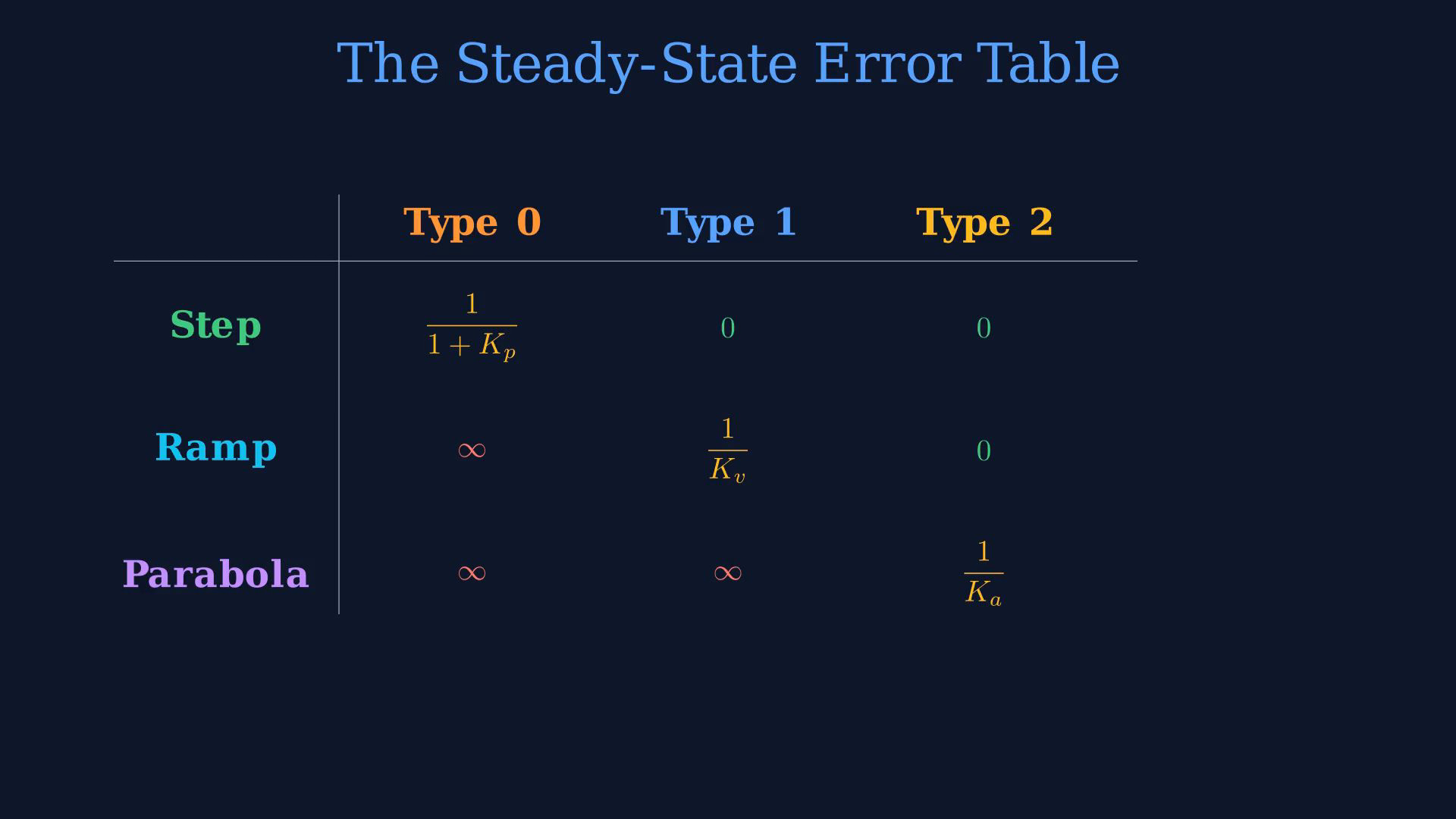
Use the stability and normalization conditions in the problem statement. Step arrows mark asymptotic gaps. System-type cards classify origin poles only. Ramp and summary sections use the existing error table as their reference; its infinity entries describe unbounded errors, not finite limits.
Read the table for stable negative unity feedback, zero initial state and normalized polynomial references.
Type-zero unit step:
$\displaystyle e_{\mathrm{ss}} =\frac{ 1}{1+K_{p}}$
Type-one and higher unit step:
$\displaystyle e_{\mathrm{ss}} = 0$
Type-zero unit ramp has unbounded error.
Type-one unit ramp:
$\displaystyle e_{\mathrm{ss}} =\frac{ 1}{K_{v}}$
Type-two and higher unit ramp:
$\displaystyle e_{\mathrm{ss}} = 0$
Type-zero and Type-one unit parabola have unbounded error.
Type-two unit parabola:
$\displaystyle e_{\mathrm{ss}} =\frac{ 1}{K_{a}}$
Type-three and higher unit parabola:
$\displaystyle e_{\mathrm{ss}} = 0$
A zero entry describes the long-time error, not the whole transient.
Rows specify the input; columns specify the net integrator count.
Narration transcript
Let us organize everything into one table. For a step input: Type zero gives error one over one plus K p. Type one and higher give zero error. For a ramp input: Type zero gives infinite error. Type one gives one over K v. Type two and higher give zero. For a parabola input: Type zero and one give infinite error. Type two gives one over K a. Type three and higher give zero. This table is the key result. Each row is an input type, each column is a system type.
8. Separate position and velocity constants
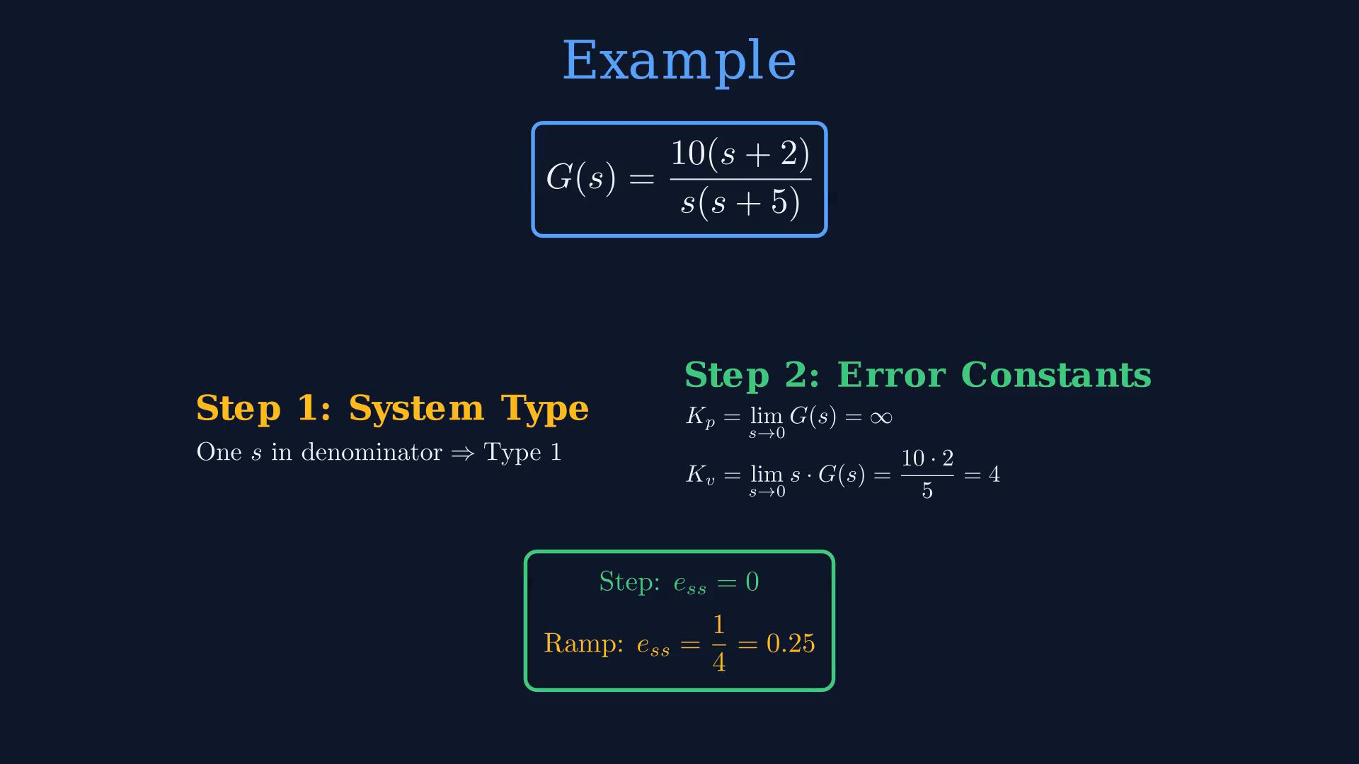
Use the stability and normalization conditions in the problem statement. Step arrows mark asymptotic gaps. System-type cards classify origin poles only. Ramp and summary sections use the existing error table as their reference; its infinity entries describe unbounded errors, not finite limits.
Work the example with negative unity feedback.
Open-loop example:
$\displaystyle G\left(s\right) = 10\cdot \frac{s+2}{s\cdot \left(s+5\right)}$
Identify the uncancelled origin pole before taking the error-constant limits.
There is one net integrator, so the example is Type one.
For the position constant Kₚ, take the limit of G(s) as s tends to zero.
The narration momentarily uses a cancellation that belongs to the velocity-constant calculation; the next sentence explicitly corrects it.
The corrected position constant is infinite because the integrator remains in G.
Taking the limit of s times G(s) as s tends to zero:
$\displaystyle K_{v} = 10\cdot \frac{2}{5 }= 4$
Stable example, unit step:
$\displaystyle e_{\mathrm{ss}} = 0$
Stable example, unit ramp:
$\displaystyle e_{\mathrm{ss}} =\frac{ 1}{4 }= 0.25$
Narration transcript
Let us work an example. Given G of s equals ten times the quantity s plus two, divided by s times the quantity s plus five. First, identify the system type. There is one s in the denominator, so this is a Type one system. K p: the limit as s goes to zero of G of s. The s cancels, giving ten times two over five, which is four. Wait, for Type one, K p is actually infinite because of the integrator. K v: the limit as s goes to zero of s times G of s equals ten times two over five, which is four. So for a step input, the error is zero. For a ramp input, the error is one over four, which is zero point two five.
9. Review the stability conditions
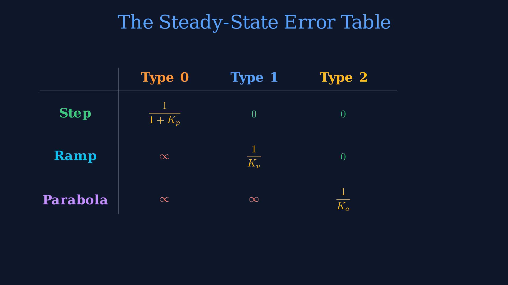
Use the stability and normalization conditions in the problem statement. Step arrows mark asymptotic gaps. System-type cards classify origin poles only. Ramp and summary sections use the existing error table as their reference; its infinity entries describe unbounded errors, not finite limits.
Review steady-state tracking.
Use input degree, system type, the relevant gain and closed-loop stability together.
Find the position, velocity and acceleration constants from the appropriate low-frequency limits.
Higher type can improve the table entry when stability is retained; an already-zero error cannot become strictly smaller.
Continue with the root locus and the motion of closed-loop poles as gain changes.
Narration transcript
To summarize. Steady state error depends on two things: the input type and the system type. The position constant K p, velocity constant K v, and acceleration constant K a are found by taking limits of G of s. The error table tells us everything: higher system type means lower error for each input. In the next lesson, we study the root locus method, which shows how closed loop poles move as we change the controller gain.