Control Theory · Step Responses

#12 Compute causal zero-state unit-step responses and distinguish lag, integrator and delay behavior

Compute step responses of four standard blocks, interpret the 63.2% time constant and check the direction of unstable divergence.

Question

Existing lesson frame illustrating a causal step, ramp, first-order response or delay equation. — Use causal zero-state unit-step inputs. The general computation card accompanies the introduction and standard-block comparison. The negative-T case uses the ODE card as an algebraic reference, not a stability plot. Distinguish positive time constant T from time t and delay Δ from the Dirac impulse.

Use continuous-time linear time-invariant input-output models with zero initial state and a causal unit-amplitude step. Sigma denotes the unit step here, not the real part of the Laplace variable. It is zero for negative time and one for positive time. The source omits its isolated value at zero; the graph chooses a right-continuous value of one. A different isolated-point convention does not change the ordinary Laplace transform or convolution integral. This does not assign a point value to a Dirac distribution. For a causal unit step, U(s) is 1/s on real part of s positive. Compute the zero-state output as G(s)/s and invert on a convergence domain consistent with causality. The phrase any transfer function presumes the transform operation exists; improper ideal transfer functions may produce distributions rather than an ordinary output curve. Nonzero initial energy contributes a separate zero-input response. For G(s)=1/s, the unit-step output is the causal ramp t times sigma(t), and its transform is 1/s squared. More generally a K/s integrator gives K times that ramp, plus any initial integrator value for nonnegative time. It has no finite steady value for nonzero K and is not BIBO stable. For a first-order lag use the constant-coefficient ODE T times the derivative of y plus y equals K times u, with T positive and K a constant. For zero initial output, the transfer function is K divided by the entire denominator one plus s times T. Distinguish the time constant T from the running time t; ASR case alone does not encode that distinction. With a unit step, partial fractions give K times the difference between 1/s and 1 divided by s plus 1/T. The causal output is K times one minus exp of minus t/T, multiplied by sigma(t). It begins at zero and approaches K asymptotically; it does not reach the exact final value in finite time. Positive K gives an increasing concave-down curve, negative K a decreasing curve, and K zero gives the identically zero zero-state output. For nonzero initial output y0, the positive-time response is K plus (y0 minus K) times exp of minus t/T. At t=T the zero-state fraction of a nonzero final value is one minus exp of minus one, approximately 0.63212056. The spoken sixty-three percent is rounded, not an exact equality. For nonzero initial state the same fraction describes the change from initial to final value, not the absolute output divided by K. Smaller positive T means faster relative-error decay for the same gain, step and initial-state convention. The curves compare T values 0.5, 1, 3 and 10 with K=1. A finite settling time requires an explicit tolerance; relative error epsilon is reached at minus T times the natural logarithm of epsilon, for epsilon strictly between zero and one. Extend the ODE algebraically to negative nonzero T only in the instability example. Its dynamic mode has pole minus 1/T in the right half-plane. For nonzero K the selected scalar transfer is BIBO unstable. The zero-state unit-step response grows without bound in magnitude: with positive K and negative T it goes toward negative infinity, not positive infinity; with negative K its direction reverses. The original phrase diverges to infinity is interpreted as unbounded magnitude, corroborated by the actual negative-going K=1 plot. Do not equate the value G(0)=K to an attained final value for this unstable model, and do not apply the final-value theorem there. A specially matched initial value can give a particular constant trajectory without making an unstable system stable. If K is zero the transfer channel vanishes but the ODE can still contain an unstable initial-state mode. If T is zero the equation degenerates to a static gain, so the positive-T requirement is for this nondegenerate first-order lag, not for every stable system. For a causal time delay take a fixed nonnegative delay Δ and zero prehistory. It shifts the time argument: y(t) is u(t minus Δ), not u(t) minus a constant. Its transfer is exp of minus Δ times s, and a unit step becomes sigma(t minus Δ). At Δ zero it is the identity. A negative Δ would describe an advance and is outside this causal-delay model. The clean delay card shows the correct minus sign and full product in the exponent; Δ is a time duration, not the Dirac impulse used in the preceding lesson. A delay stores input history and is not a finite-dimensional rational transfer except at zero delay or under a stated approximation. The four listed blocks are common modeling elements with appropriate summing and interconnection rules. They are not an exhaustive theorem for every linear system: arbitrary time-varying or distributed-parameter systems need additional structure, and a differentiation operator is not included in this four-block list. Qualify stability, causality, initial state, step amplitude and transform existence before using the response formulas. These plant examples do not by themselves provide a controller design or a tracking guarantee.

Written solution and narration transcript(shows the full solution)

Below are all the lines written in the notebook together with the full narration transcript.

1. Introduce step responses
Use causal zero-state unit-step inputs. The general computation card accompanies the introduction and standard-block comparison. The negative-T case uses the ODE card as an algebraic reference, not a stability plot. Distinguish positive time constant T from time t and delay Δ from the Dirac impulse.
Introduce Control Theory, Lesson 12.
Recall impulse response and convolution.
Use step responses to analyze the specified LTI zero-state channel.
Compare an integrator, first-order lag and causal delay.
Narration transcript
Welcome to lesson twelve. Last time we learned about impulse response and convolution. Today we study the step response, one of the most important tools for analyzing system behavior. We will compute step responses for the integrator, the first-order lag, and the time delay.
2. Define the causal unit step
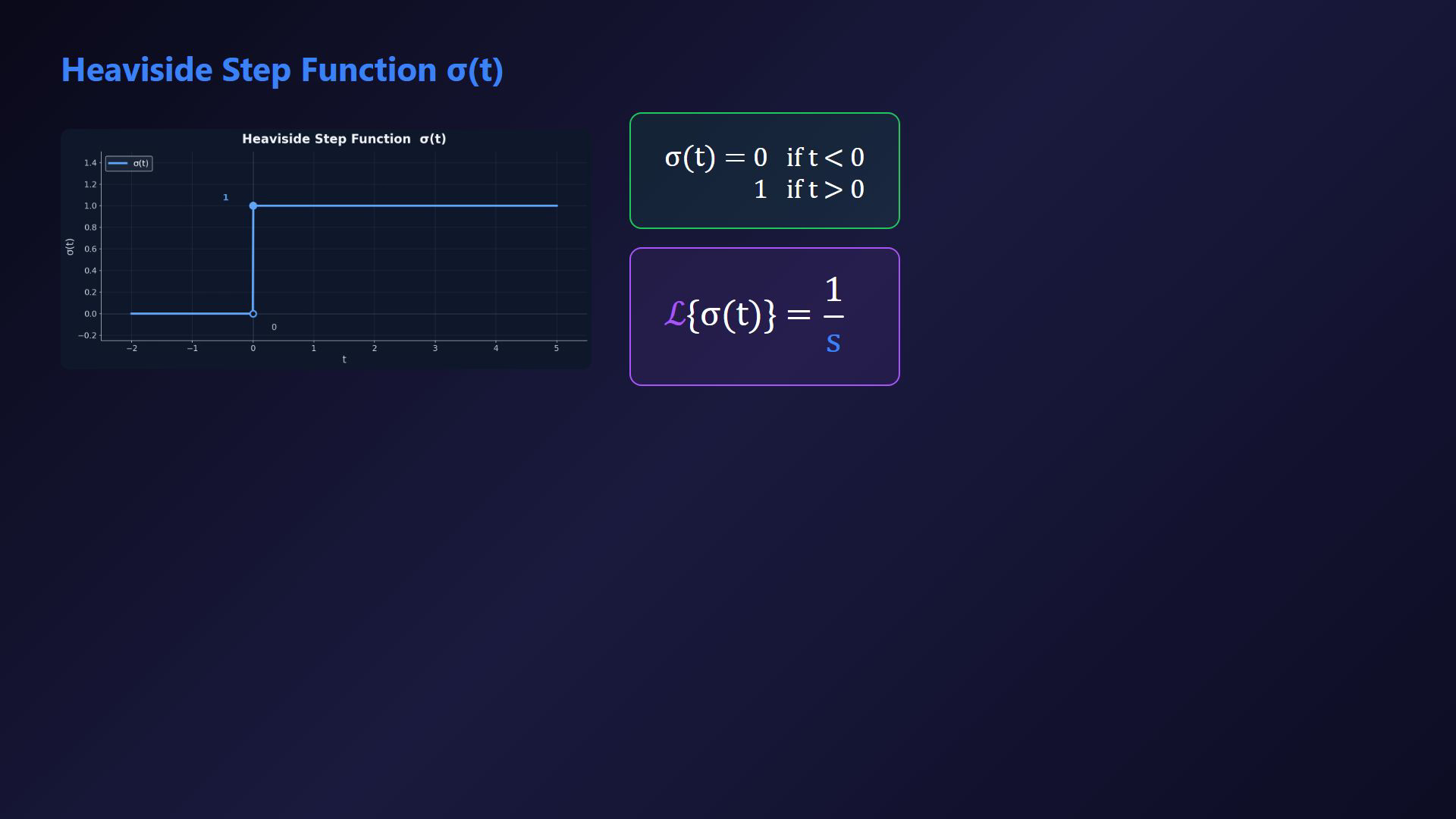
Use causal zero-state unit-step inputs. The general computation card accompanies the introduction and standard-block comparison. The negative-T case uses the ODE card as an algebraic reference, not a stability plot. Distinguish positive time constant T from time t and delay Δ from the Dirac impulse.
The unit step σ(t) is zero for negative time and one for positive time.
Switch on a unit-amplitude constant input at zero.
Causal step transform:
$\displaystyle L\{\sigma \left(t\right)\} =\frac{ 1}{s}$
Define the zero-state unit-step response as the output for this input.
Narration transcript
The Heaviside step function sigma of t is zero for negative time and one for positive time. It represents switching on a constant input at time zero. Its Laplace transform is one over s. The step response of a system is the output when this function is applied as input.
3. Compute a zero-state step response
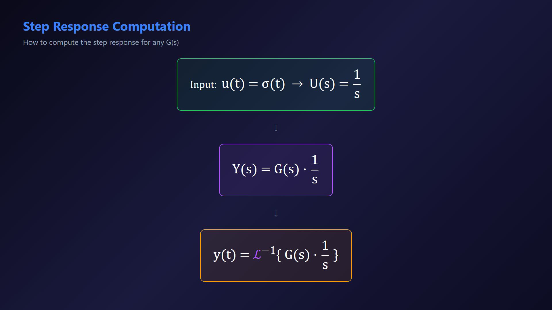
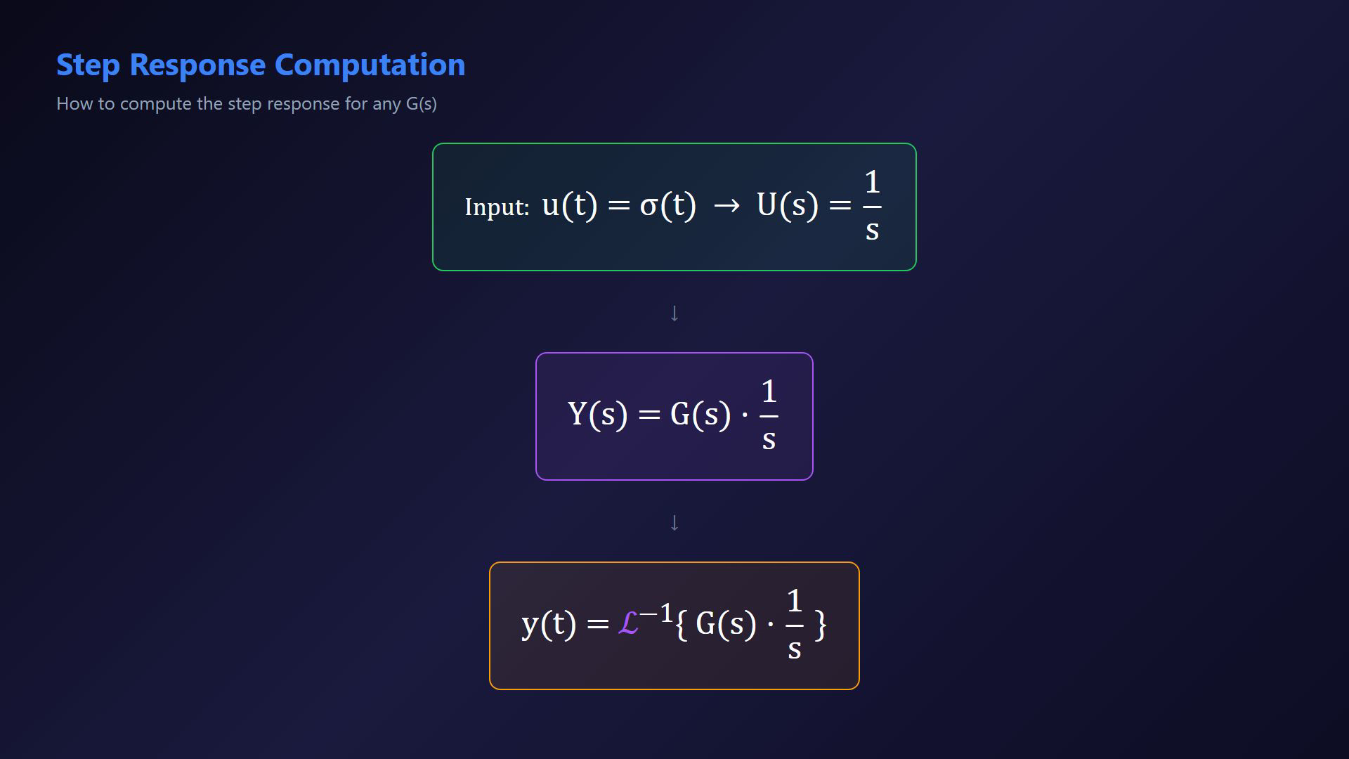
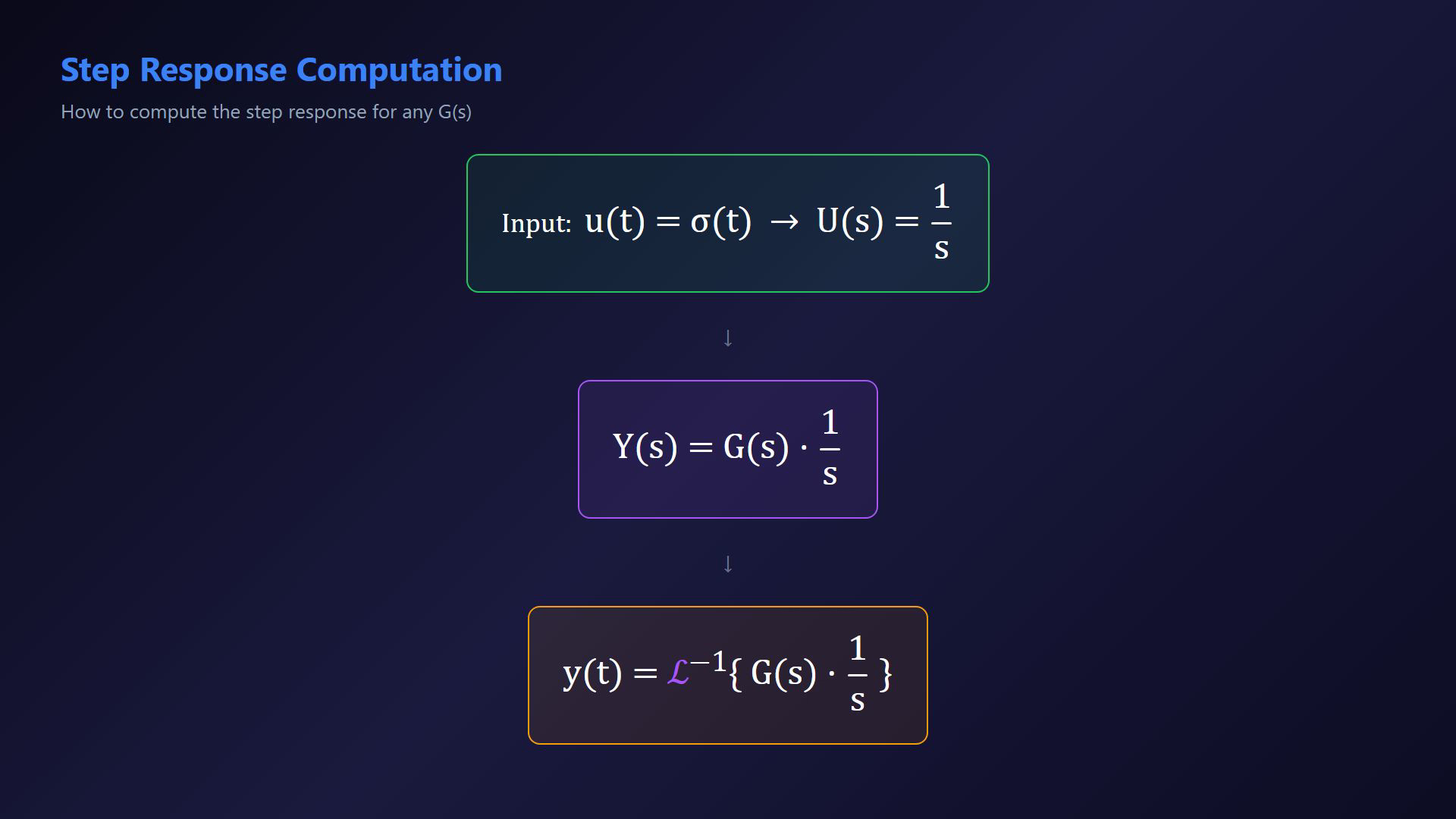
Use causal zero-state unit-step inputs. The general computation card accompanies the introduction and standard-block comparison. The negative-T case uses the ODE card as an algebraic reference, not a stability plot. Distinguish positive time constant T from time t and delay Δ from the Dirac impulse.
Unit-step input transform:
$\displaystyle U\left(s\right) =\frac{ 1}{s}$
Zero-state output transform:
$\displaystyle Y\left(s\right) =\frac{ G\left(s\right)}{s}$
Inverse transform on the causal branch:
$\displaystyle y\left(t\right) = L^{-1}\{G\left(s\right)/s\}$
Use the procedure where the transforms and inverse are defined.
Narration transcript
To compute the step response, we set U of s equal to one over s. Then Y of s equals G of s times one over s. To get y of t, we take the inverse Laplace transform of G of s divided by s. This is the standard procedure for any transfer function.
4. Check the integrator ramp
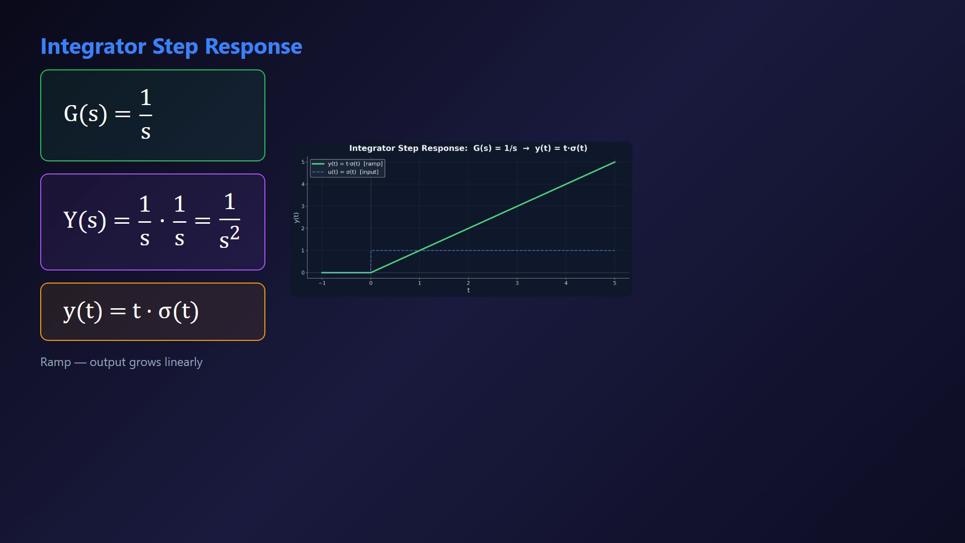
Use causal zero-state unit-step inputs. The general computation card accompanies the introduction and standard-block comparison. The negative-T case uses the ODE card as an algebraic reference, not a stability plot. Distinguish positive time constant T from time t and delay Δ from the Dirac impulse.
Pure integrator:
$\displaystyle G\left(s\right) =\frac{ 1}{s}$
Unit-step output transform:
$\displaystyle Y\left(s\right) = 1/s²$
Causal ramp response:
$\displaystyle y\left(t\right) = t\cdot \sigma \left(t\right)$
A zero-state unit-gain integrator accumulates the constant unit input.
Narration transcript
The simplest example is the pure integrator with G of s equals one over s. The step response becomes Y of s equals one over s squared. Taking the inverse Laplace transform, we get y of t equals t times sigma of t, which is a ramp. The integrator accumulates the constant input, so the output grows linearly with time.
5. Derive the first-order transfer
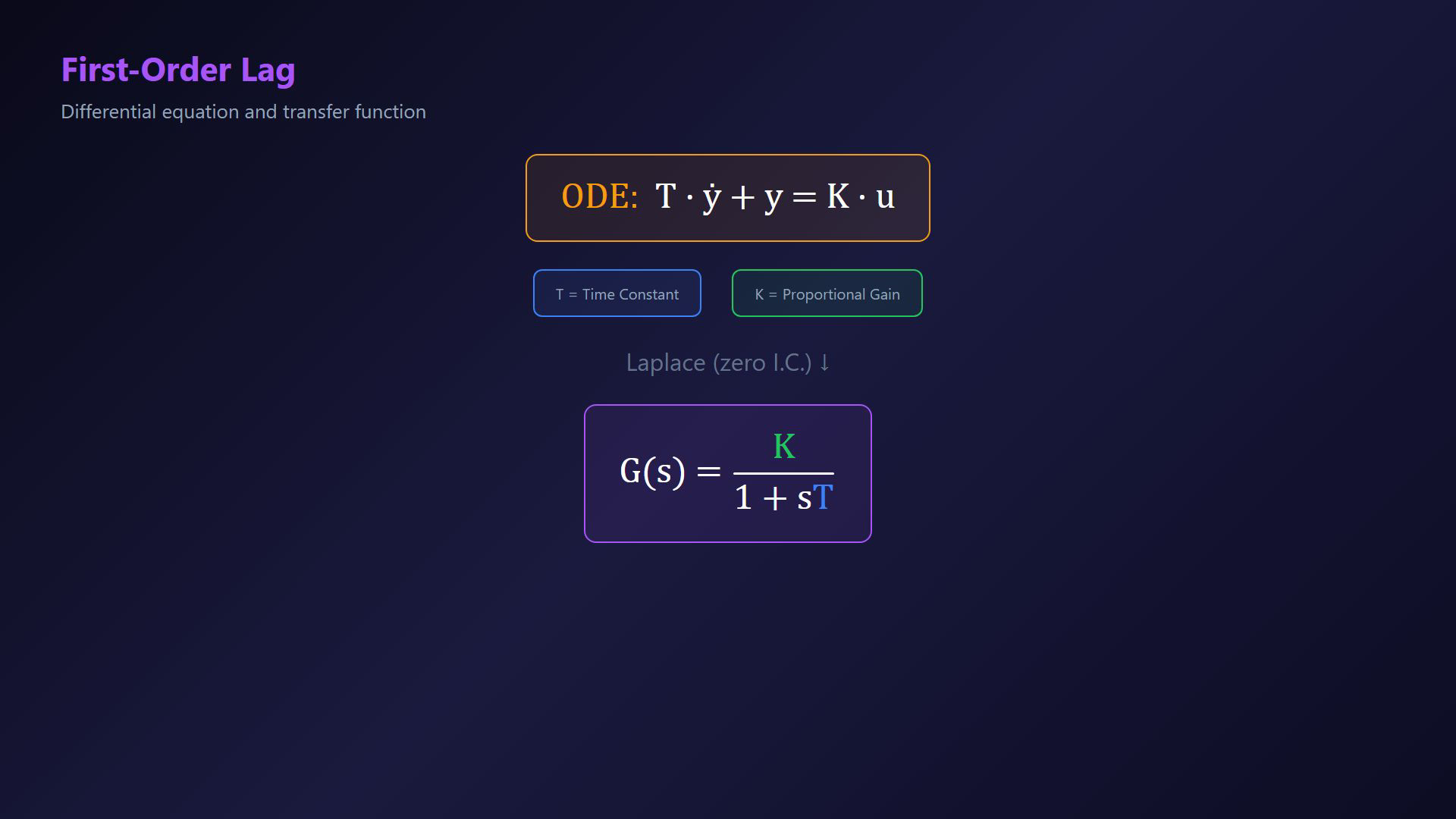
Use causal zero-state unit-step inputs. The general computation card accompanies the introduction and standard-block comparison. The negative-T case uses the ODE card as an algebraic reference, not a stability plot. Distinguish positive time constant T from time t and delay Δ from the Dirac impulse.
Study a first-order lag with constant positive T.
First-order ODE:
$\displaystyle T\cdot y'\left(t\right) + y\left(t\right) = K\cdot u\left(t\right)$
Distinguish the time constant T and gain K from time t.
Zero-initial-state transfer:
$\displaystyle G\left(s\right) =\frac{ K}{1+s\cdot T}$
Narration transcript
Next we study the first-order lag. Its differential equation is T times y dot plus y equals K times u. Here T is the time constant and K is the proportional gain. Taking the Laplace transform with zero initial conditions, the transfer function becomes G of s equals K over one plus s T.
6. Invert the first-order step transform
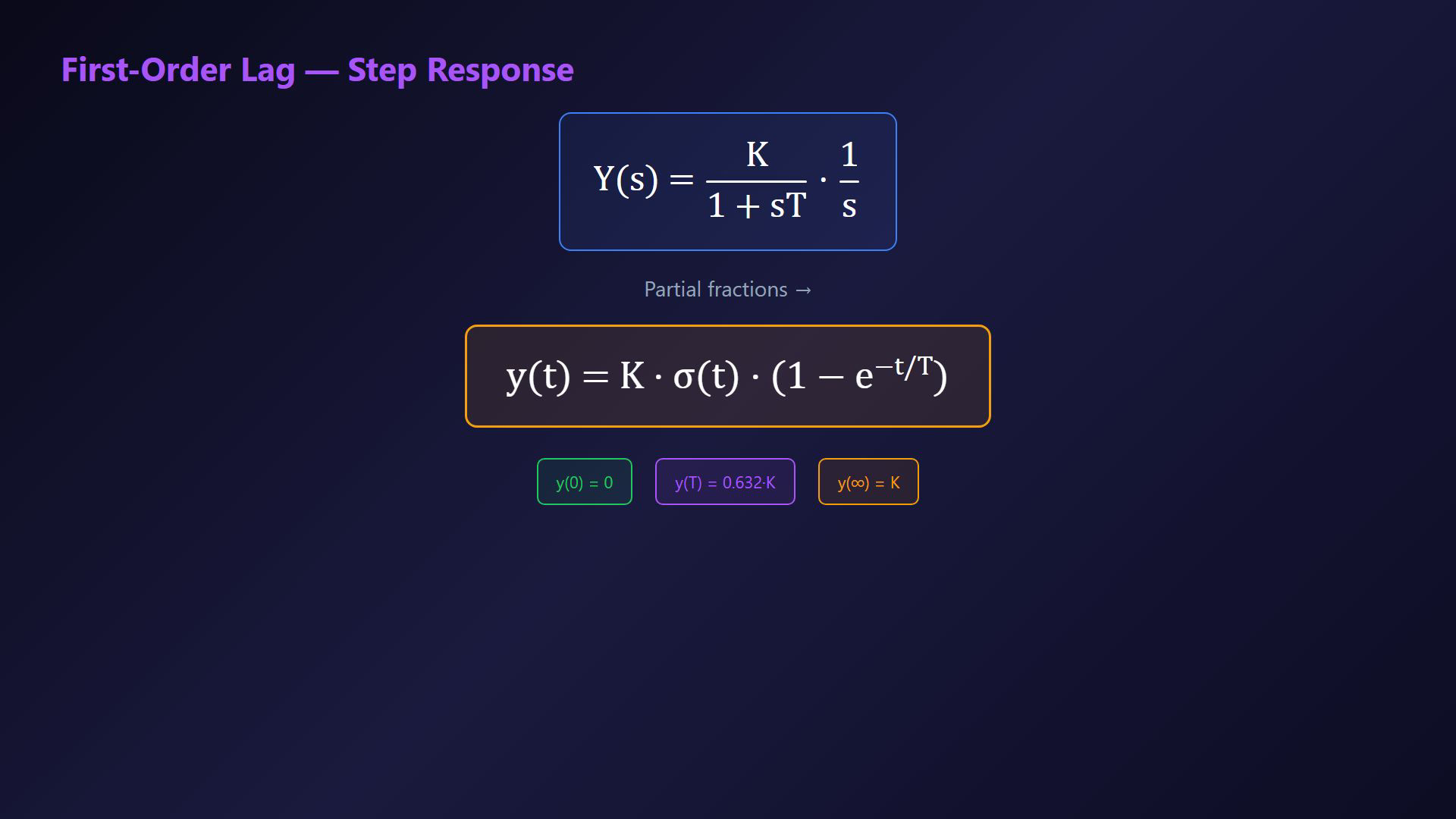
Use causal zero-state unit-step inputs. The general computation card accompanies the introduction and standard-block comparison. The negative-T case uses the ODE card as an algebraic reference, not a stability plot. Distinguish positive time constant T from time t and delay Δ from the Dirac impulse.
Step transform:
$\displaystyle Y\left(s\right) = \left(\frac{K}{1+s\cdot T}\right)\cdot \left(\frac{1}{s}\right)$
Causal first-order response:
$\displaystyle y\left(t\right) = K\cdot \sigma \left(t\right)\cdot \left(1-e^{-t/T}\right)$
For positive T, start at zero and approach K asymptotically.
Narration transcript
To find the step response, we compute Y of s equals K over one plus s T times one over s. Using partial fraction decomposition, we get y of t equals K times sigma of t times one minus e to the minus t over T. The output starts at zero and exponentially approaches the final value K.
7. Compare positive time constants
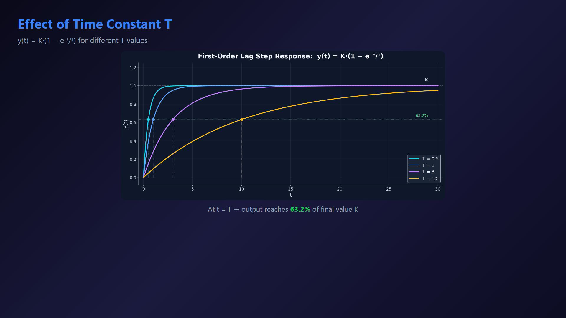
Use causal zero-state unit-step inputs. The general computation card accompanies the introduction and standard-block comparison. The negative-T case uses the ODE card as an algebraic reference, not a stability plot. Distinguish positive time constant T from time t and delay Δ from the Dirac impulse.
Compare positive time constants with the same gain and unit step.
A time constant of 0.5 gives faster relative-error decay.
Time constants of 3 or 10 give slower responses.
At one time constant:
$\displaystyle y\left(T\right) = K\cdot \left(1-e^{-1}\right) \approx 0.63212\cdot K$
Apply this fraction to the zero-state first-order lag; finite settling needs a tolerance.
Narration transcript
Let us see how the time constant T affects the response. For small T like zero point five, the system responds quickly and reaches steady state fast. For larger T like three or ten, the response is slower. In all cases, the output reaches sixty-three percent of the final value at time t equals T. This is a key property of first-order systems.
8. Examine the unstable negative-T case
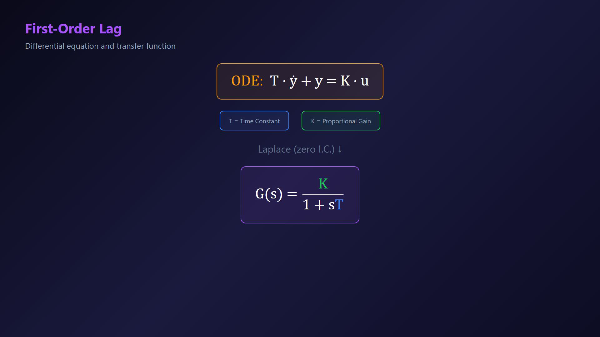
Use causal zero-state unit-step inputs. The general computation card accompanies the introduction and standard-block comparison. The negative-T case uses the ODE card as an algebraic reference, not a stability plot. Distinguish positive time constant T from time t and delay Δ from the Dirac impulse.
Extend the model to a negative nonzero T for the instability example.
Dynamic pole:
$\displaystyle p = -\frac{1}{T}$
For positive K and negative T, the unit-step output diverges toward negative infinity.
The negative-T dynamic mode is unstable; a nonzero-K transfer exposes it.
The nondegenerate stable first-order lag has positive T.
Narration transcript
What happens when the time constant T is negative? The transfer function still looks the same, K over one plus s T, but now the pole is in the right half of the s-plane. The response diverges to infinity instead of settling. A negative time constant means the system is unstable. Stability requires T greater than zero.
9. Apply a causal time delay
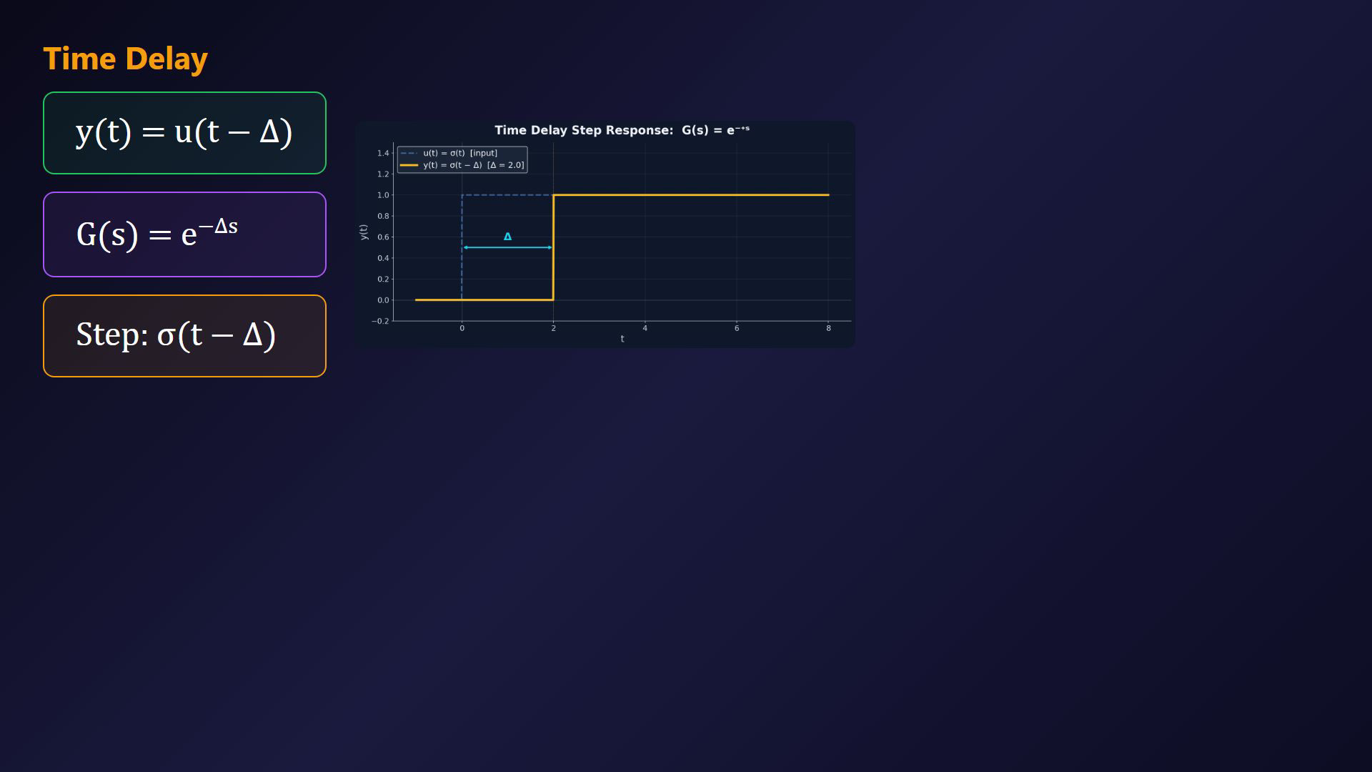
Use causal zero-state unit-step inputs. The general computation card accompanies the introduction and standard-block comparison. The negative-T case uses the ODE card as an algebraic reference, not a stability plot. Distinguish positive time constant T from time t and delay Δ from the Dirac impulse.
Use a fixed nonnegative delay Δ and zero prehistory.
Shift the input time argument by Δ.
Time-delay relation:
$\displaystyle y\left(t\right) = u\left(t-\Delta \right)$
Delay transfer:
$\displaystyle G\left(s\right) = e^{-\Delta \cdot s}$
Delayed unit step:
$\displaystyle y\left(t\right) = \sigma \left(t-\Delta \right)$
Narration transcript
The time delay is a special transfer block. The output equals the input shifted by delta time units. So y of t equals u of t minus delta. The transfer function is G of s equals e to the minus delta s. Applying a step input, the step response is simply a delayed step that jumps from zero to one at time t equals delta.
10. Compare the standard transfer blocks
Use causal zero-state unit-step inputs. The general computation card accompanies the introduction and standard-block comparison. The negative-T case uses the ODE card as an algebraic reference, not a stability plot. Distinguish positive time constant T from time t and delay Δ from the Dirac impulse.
Compare four common transfer blocks under the stated assumptions.
Proportional block:
$\displaystyle G\left(s\right) = K, y\left(t\right) = K\cdot \sigma \left(t\right)$
Integrator block:
$\displaystyle G\left(s\right) =\frac{ K}{s}, y\left(t\right) = K\cdot t\cdot \sigma \left(t\right)$
Positive-T lag:
$\displaystyle G\left(s\right) =\frac{ K}{1+s\cdot T}, y\left(t\right) = K\cdot \left(1-e^{-t/T}\right)\cdot \sigma \left(t\right)$
Causal delay:
$\displaystyle G\left(s\right) = e^{-\Delta \cdot s}, y\left(t\right) = \sigma \left(t-\Delta \right)$
These common elements require suitable interconnections and do not exhaust all linear systems.
Narration transcript
Let us summarize the four standardized transfer blocks. Proportional gain K, with step response K sigma of t. The integrator K over s, with step response K t sigma of t, a ramp. The first-order lag K over one plus s T, with step response K times one minus e to the minus t over T. And the time delay e to the minus delta s, with step response sigma of t minus delta. These are the building blocks for modeling any linear system.
11. Review the response assumptions
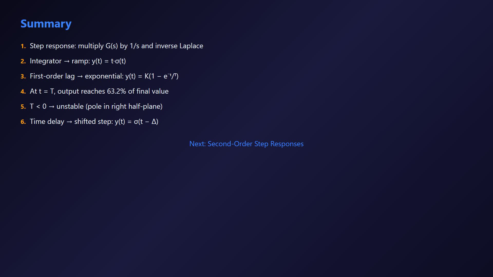
Use causal zero-state unit-step inputs. The general computation card accompanies the introduction and standard-block comparison. The negative-T case uses the ODE card as an algebraic reference, not a stability plot. Distinguish positive time constant T from time t and delay Δ from the Dirac impulse.
Review the result.
Compute a defined zero-state step response by dividing G(s) by s and inverting.
Compare the integrator ramp and the stable positive-T exponential response.
A negative-T dynamic mode is unstable, with the stated channel qualifications.
A causal delay shifts the step by nonnegative Δ.
Continue with second-order step responses.
Narration transcript
Excellent work. In this lesson we learned that the step response is computed by multiplying G of s with one over s and taking the inverse Laplace transform. The integrator gives a ramp, the first-order lag gives an exponential rise toward K, with time constant T determining the speed. A negative T means instability. And the time delay simply shifts the step by delta. Next we will study second-order step responses.