Control Theory · The Transfer Function Concept

#10 Derive zero-state transfer functions from constant-coefficient LTI differential equations

Connect differential equations to transfer blocks, distinguish properness and reduced order, and derive parallel RC, RLC and motor models.

Question

Existing lesson frame illustrating a system operator, Laplace equation or transfer-function definition. — Read the formulas in the finite-dimensional LTI and zero-initial-state setting. The RC and RLC examples use the general transfer-function definition card; the motor uses the general LTI equation card. The integrator comparison uses the Laplace operator card. These are algebraic references, not physical circuit wiring or a completed motor diagram. Count transfer-function order after cancellation of common polynomial factors.

Restrict this lesson to finite-dimensional continuous-time linear time-invariant models with constant coefficients and rational transfer functions. A general system operator maps the whole input history to output history once the initial state is specified; the notation S acting on u(t) does not imply a memoryless map. The source statement every linear system can be built from the three listed operators is too broad without this scope: finite interconnections of constant gains, integrators, differentiators and signed sums describe rational constant-coefficient ODE models, not arbitrary time-varying or distributed-delay linear systems. A pure time delay has an exponential transfer function and needs a delay element or an explicitly stated approximation. Ideal differentiation also requires suitable input regularity and is not a bounded high-frequency physical gain. The zero-state integrator starts from zero; a nonzero initial integral value adds a constant. The unilateral Laplace transform of a derivative includes the initial value. Multiplication by s alone requires the appropriate zero-initial-value assumption, explicitly stated in the ODE scene. Higher derivatives carry all corresponding initial terms; integrals use the same lower limit. Use causal zero-state signals, including any input-derivative impulse at switch-on when needed. For the constant-coefficient ODE, define the output polynomial A(s) and input polynomial B(s). Then A(s) times Y(s) equals B(s) times U(s), and the transfer function is B(s) divided by A(s). The notation Y(s)/U(s) is the zero-state operator ratio where that quotient is defined; it is not evaluated as zero divided by zero for a zero input and does not by itself include the zero-input response from stored energy. Cancel common factors before calling denominator degree the transfer-function order. An unreduced differential equation may have higher order and hidden internal modes; a canceled unstable mode is not proof of internal stability. For a nonzero rational transfer function with nonzero leading coefficients, relative degree is denominator degree minus numerator degree. Strictly proper means positive relative degree; proper includes both positive and zero relative degree; zero relative degree is the biproper special case. The source zero-relative-degree statement is sufficient for properness, not its only case; the actual properties card states greater than or equal to zero. These algebraic classifications alone do not prove stability or practical realizability. The RC example is a parallel resistor-capacitor driven by input current u with common output voltage y. Its current balance is C times the derivative of y plus y/R equals u. The transfer denominator is the whole sum s times C plus 1/R, with positive constant R and C. Its DC voltage/current gain is R and time constant is RC. The RLC example is the corresponding parallel network with common voltage y and inductor current as an additional state. Differentiating its KCL gives C times the second derivative of y plus the first derivative divided by R plus y/L equals the first derivative of u. Initial inductor current and capacitor voltage must remain compatible with the undifferentiated KCL. With zero stored energy the transfer function is s divided by the whole sum C times s squared plus s/R plus 1/L. These are impedances, not the transfer laws of a series sketch. The general equation cards are algebraic references for these examples. For the DC motor, denote the fixed coupling coefficient spoken as c phi F by K; do not turn phi into the number five or infer an extra independent force input from the trailing F notation. Use consistent units for the same ideal back-EMF and torque coefficient. The electrical integrator gain is 1 divided by the entire product L_a times s; the mechanical one is 1 divided by J times s. The resistive voltage R_a times current and back EMF K times speed must be separate negative terms in the electrical sum. They cannot be merged as two output signals on an unlabeled wire. Motor torque K times current enters the mechanical sum positively and opposing load torque negatively. Friction is omitted in this ideal model. No loop can be replaced independently while ignoring coupling to the other loop. For zero initial states and zero load-torque input, eliminating current gives speed/voltage numerator K and denominator J times L_a times s squared plus J times R_a times s plus K squared. For nonzero load torque there is a second input contribution with numerator minus the sum L_a times s plus R_a over that same denominator. The voltage transfer alone does not predict arbitrary load-disturbance response. Retain both independent initial states when they are nonzero. The motor equation card is an algebraic reference, not a complete block diagram. Replacing integrators by 1/s preserves an otherwise correct zero-state signal graph and constant gains; it cannot repair a missing signed sum. The module introduces modeling, not a separate controller design or a tracking guarantee.

Written solution and narration transcript(shows the full solution)

Below are all the lines written in the notebook together with the full narration transcript.

1. Introduce transfer functions
Read the formulas in the finite-dimensional LTI and zero-initial-state setting. The RC and RLC examples use the general transfer-function definition card; the motor uses the general LTI equation card. The integrator comparison uses the Laplace operator card. These are algebraic references, not physical circuit wiring or a completed motor diagram. Count transfer-function order after cancellation of common polynomial factors.
Introduce the transfer-function concept.
Continue with Control Theory, Lesson 10.
Describe zero-state input-output behavior of a finite-dimensional LTI model.
Narration transcript
Hello everyone. Welcome to lesson ten of our control theory course. In this lesson, we introduce the transfer function, a powerful tool that describes the input-output behavior of a linear system in the Laplace domain.
2. Define the system operator
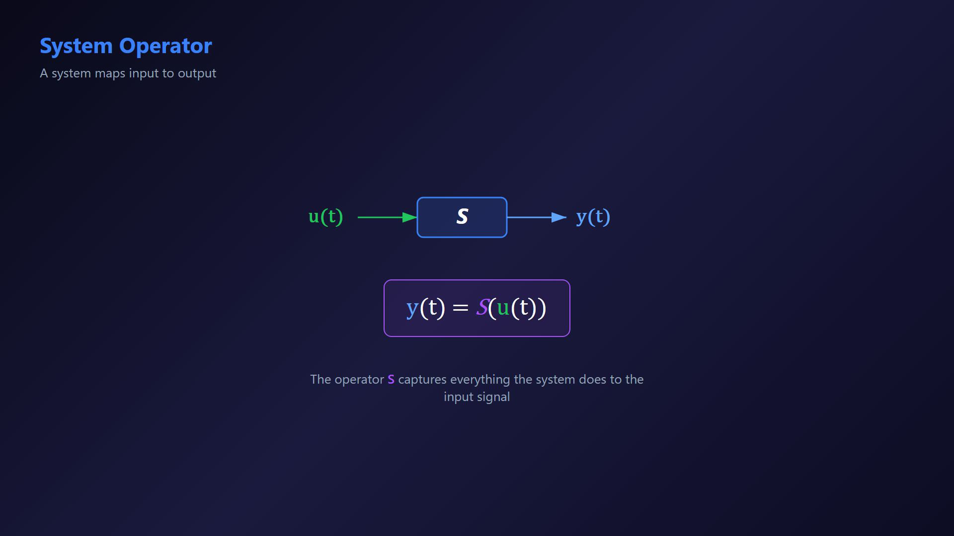
Read the formulas in the finite-dimensional LTI and zero-initial-state setting. The RC and RLC examples use the general transfer-function definition card; the motor uses the general LTI equation card. The integrator comparison uses the Laplace operator card. These are algebraic references, not physical circuit wiring or a completed motor diagram. Count transfer-function order after cancellation of common polynomial factors.
Map an input history to an output history with a specified initial state.
Operator notation:
$\displaystyle y\left(t\right) = S\left(u\left(t\right)\right).$
The operator may include memory and dynamics.
Narration transcript
Every dynamic system maps an input signal u of t to an output signal y of t. We write this as y of t equals S of u of t, where S is the system operator. The operator captures everything the system does to the input.
3. Review three basic operators
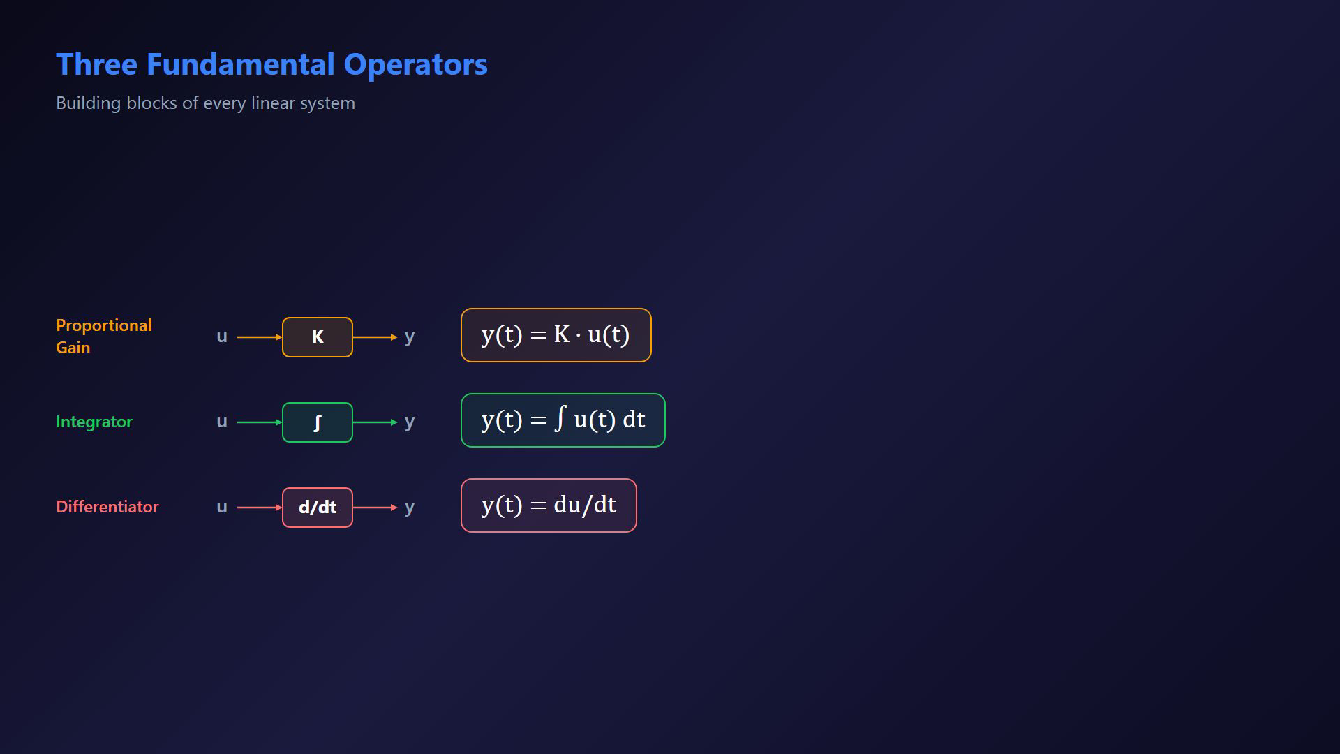
Read the formulas in the finite-dimensional LTI and zero-initial-state setting. The RC and RLC examples use the general transfer-function definition card; the motor uses the general LTI equation card. The integrator comparison uses the Laplace operator card. These are algebraic references, not physical circuit wiring or a completed motor diagram. Count transfer-function order after cancellation of common polynomial factors.
Review three elementary operators and the required signed sums.
Constant gain:
$\displaystyle y\left(t\right) = K\cdot u\left(t\right).$
Zero-state integrator:
$\displaystyle y\left(t\right) = \int u\left(t\right) \mathrm{d}t.$
Ideal differentiator:
$\displaystyle y\left(t\right) = u'\left(t\right).$
Use these blocks for rational constant-coefficient LTI ODE models; arbitrary linear systems need not fit this scope.
Narration transcript
There are three fundamental operators. First, proportional gain, where y equals K times u. Second, the integrator, where y equals the integral of u. And third, the differentiator, where y equals the derivative of u. Every linear system can be built from these basic blocks.
4. Move to the Laplace domain
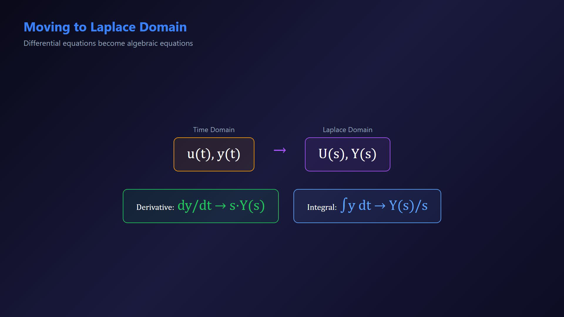
Read the formulas in the finite-dimensional LTI and zero-initial-state setting. The RC and RLC examples use the general transfer-function definition card; the motor uses the general LTI equation card. The integrator comparison uses the Laplace operator card. These are algebraic references, not physical circuit wiring or a completed motor diagram. Count transfer-function order after cancellation of common polynomial factors.
Move from time signals to their Laplace transforms.
Use the complex Laplace variable s on a domain where the transforms exist.
With the stated zero initial values, differentiation multiplies by s and integration divides by s.
The constant-coefficient ODE becomes an algebraic relation.
Narration transcript
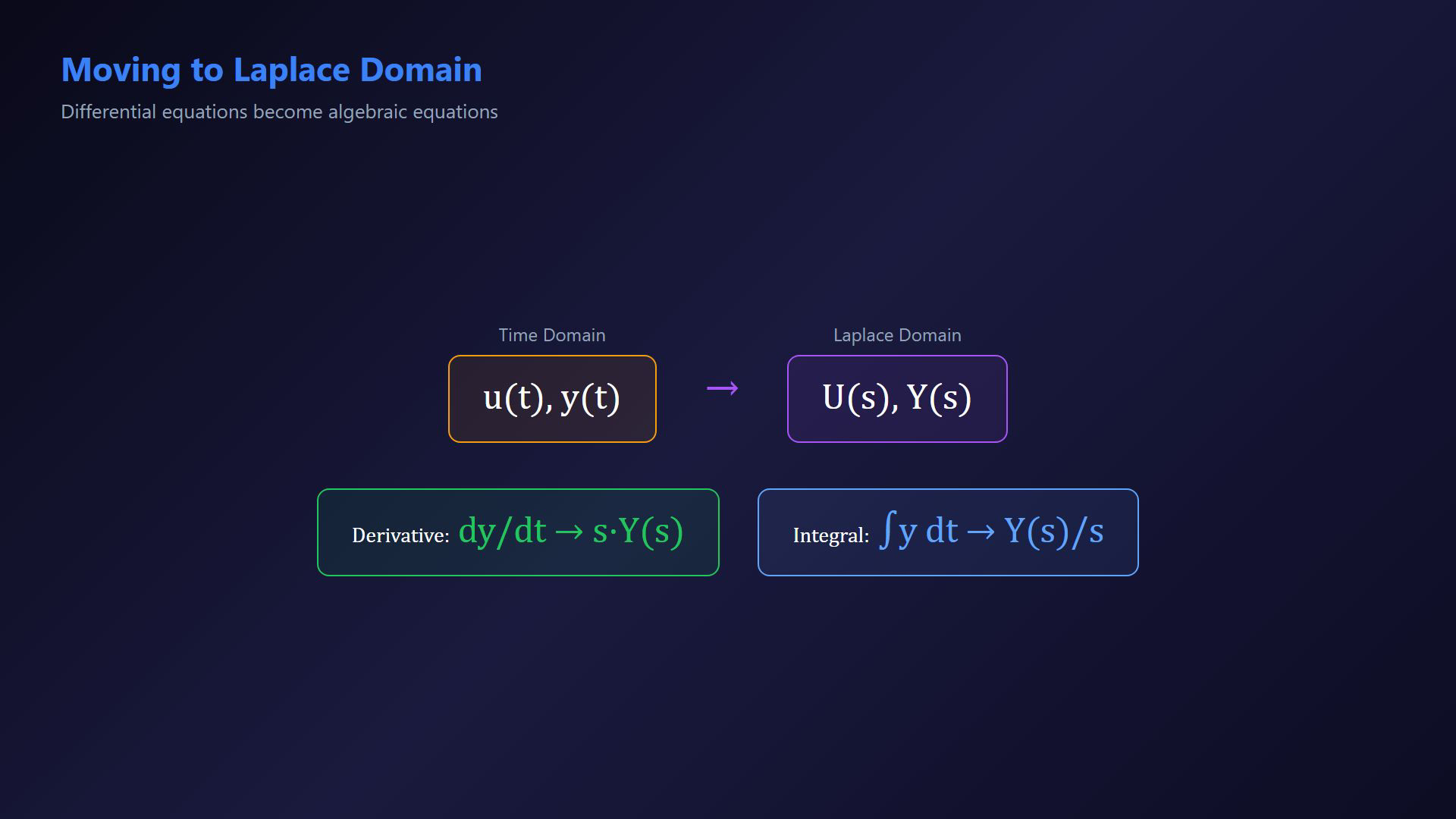
Now we move from the time domain to the Laplace domain. Recall that the Laplace transform converts a time function into a function of the complex variable s. A derivative becomes multiplication by s, and an integral becomes division by s. This turns differential equations into algebraic equations.
5. Transform the LTI differential equation
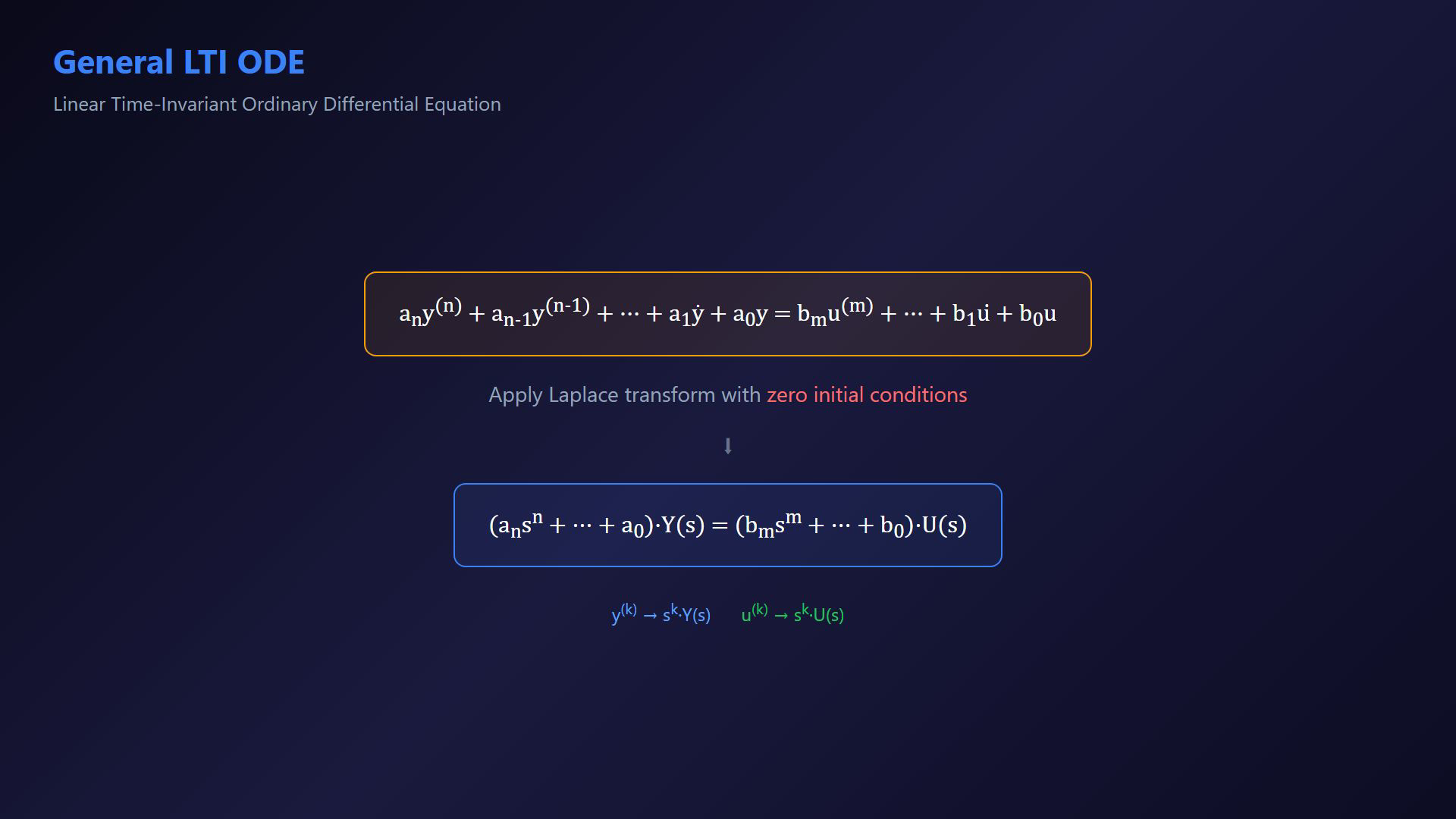
Read the formulas in the finite-dimensional LTI and zero-initial-state setting. The RC and RLC examples use the general transfer-function definition card; the motor uses the general LTI equation card. The integrator comparison uses the Laplace operator card. These are algebraic references, not physical circuit wiring or a completed motor diagram. Count transfer-function order after cancellation of common polynomial factors.
Start with a finite-order constant-coefficient LTI ODE.
Define output order n and input-derivative order m with nonzero leading coefficients.
Apply the transform with all required zero initial conditions.
Narration transcript
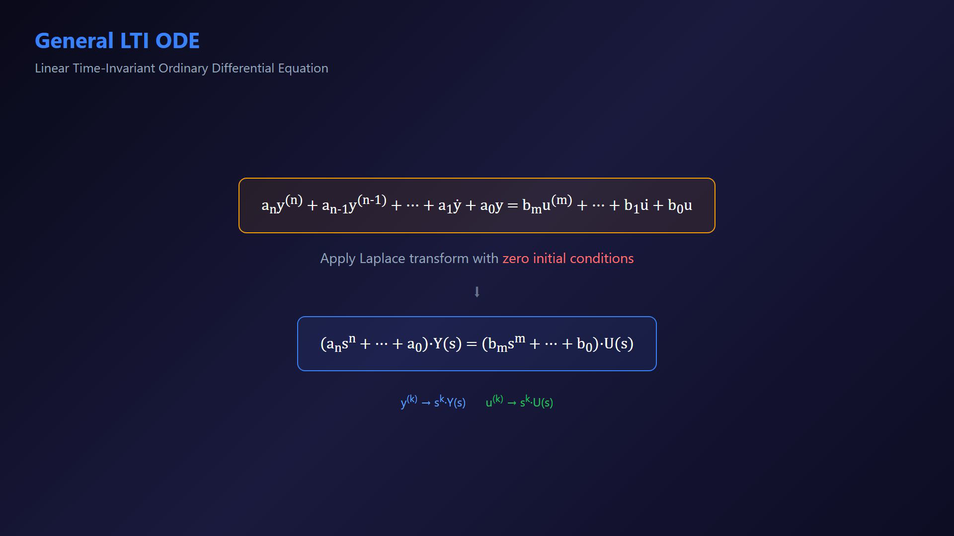
Consider a general linear time-invariant ODE. The left side has output derivatives up to order n, and the right side has input derivatives up to order m. Applying the Laplace transform with zero initial conditions, every derivative of y becomes a power of s times Y of s, and similarly for the input side.
6. Define the zero-state transfer function
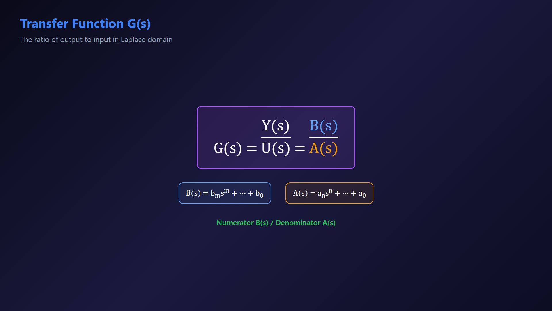
Read the formulas in the finite-dimensional LTI and zero-initial-state setting. The RC and RLC examples use the general transfer-function definition card; the motor uses the general LTI equation card. The integrator comparison uses the Laplace operator card. These are algebraic references, not physical circuit wiring or a completed motor diagram. Count transfer-function order after cancellation of common polynomial factors.
Factor the transforms:
$\displaystyle A\left(s\right)\cdot Y\left(s\right) = B\left(s\right)\cdot U\left(s\right).$
Zero-state transfer ratio:
$\displaystyle G\left(s\right) = Y\left(s\right)/U\left(s\right).$
Polynomial form:
$\displaystyle G\left(s\right) = B\left(s\right)/A\left(s\right).$
Narration transcript
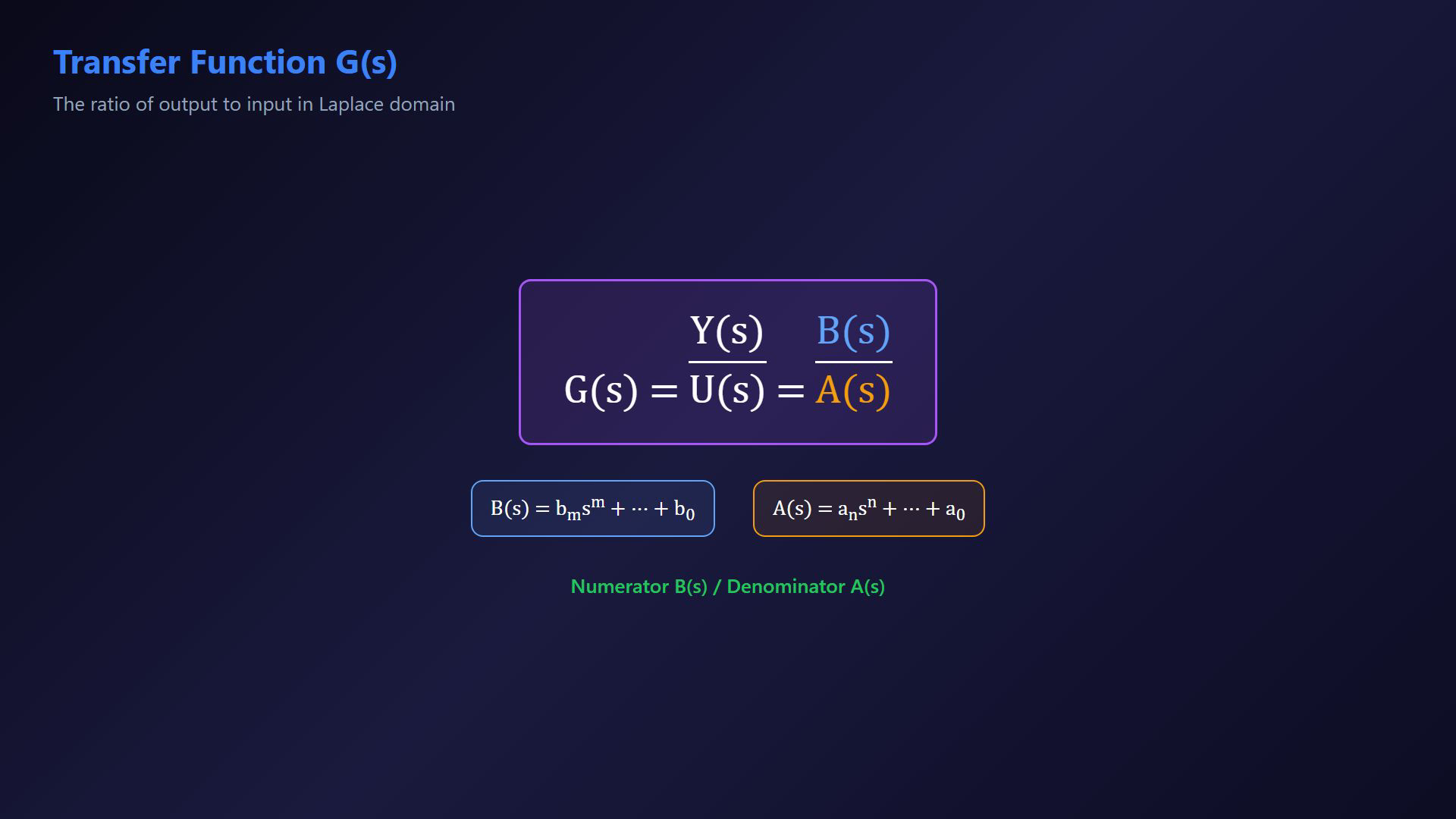
After Laplace transformation, we can factor out Y of s on the left and U of s on the right. The ratio Y of s divided by U of s gives us the transfer function G of s. It equals B of s over A of s, where B is the numerator polynomial and A is the denominator polynomial.
7. Read the transfer block
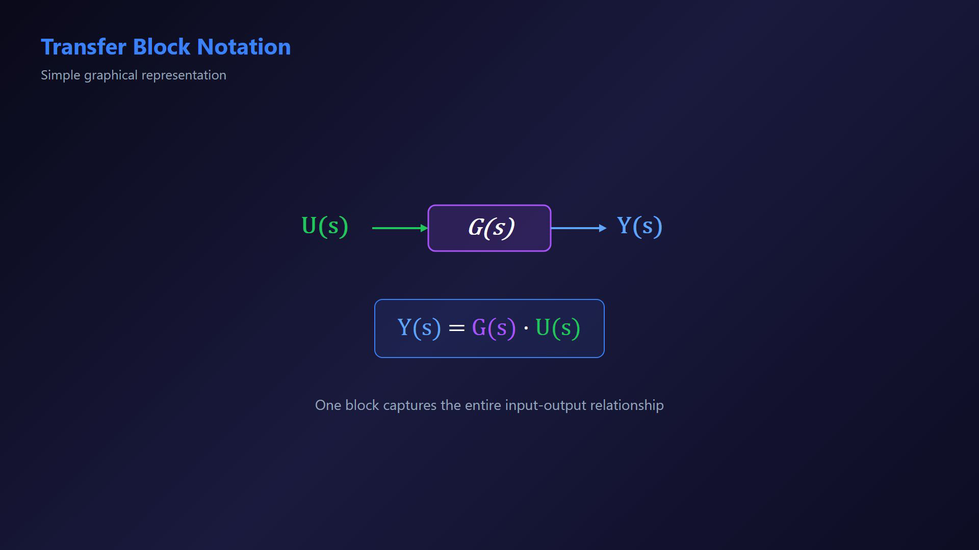
Read the formulas in the finite-dimensional LTI and zero-initial-state setting. The RC and RLC examples use the general transfer-function definition card; the motor uses the general LTI equation card. The integrator comparison uses the Laplace operator card. These are algebraic references, not physical circuit wiring or a completed motor diagram. Count transfer-function order after cancellation of common polynomial factors.
Represent the zero-state relation by a transfer block.
Send U(s) into G(s) and label its output Y(s).
The block describes the selected input-output channel.
Transfer relation:
$\displaystyle Y\left(s\right) = G\left(s\right)\cdot U\left(s\right).$
Narration transcript
We represent the transfer function as a block diagram. Input U of s enters a rectangular block labeled G of s, and the output Y of s exits. This simple notation tells us the complete input-output relationship. The output is simply G of s times U of s.
8. Distinguish order and relative degree
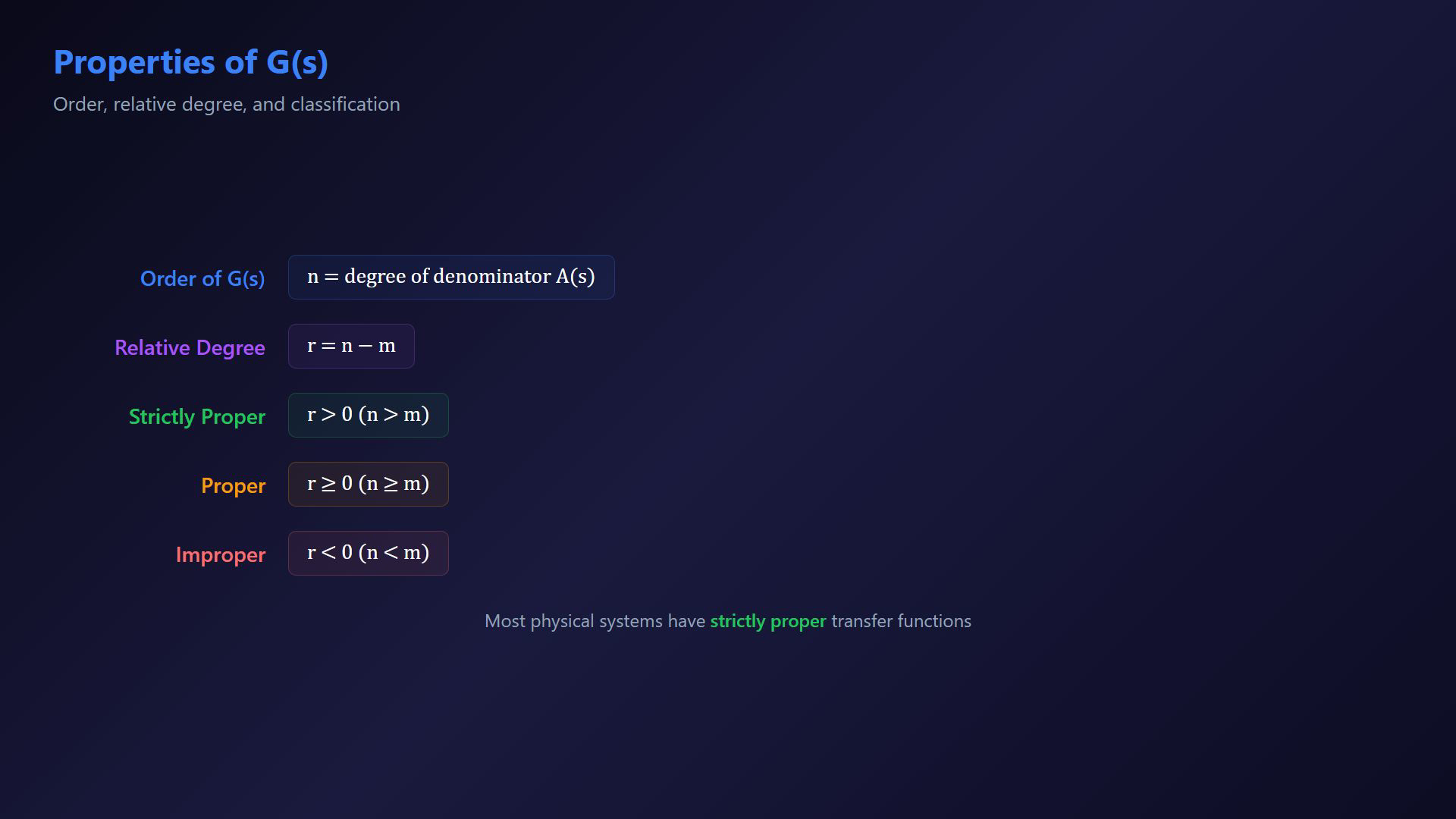
Read the formulas in the finite-dimensional LTI and zero-initial-state setting. The RC and RLC examples use the general transfer-function definition card; the motor uses the general LTI equation card. The integrator comparison uses the Laplace operator card. These are algebraic references, not physical circuit wiring or a completed motor diagram. Count transfer-function order after cancellation of common polynomial factors.
Classify a nonzero rational transfer function.
Count denominator degree after canceling common factors.
Relative degree:
$\displaystyle r = n - m.$
Positive relative degree means strictly proper.
Zero relative degree is proper; proper also includes strictly proper cases.
Properness alone does not establish stability or physical realizability.
Narration transcript
A few important properties. The order of the transfer function is n, the degree of the denominator. The relative degree is n minus m. If the relative degree is positive, the transfer function is strictly proper. If it is zero, the function is proper. Proper and strictly proper transfer functions are the most common in practice.
9. Derive the parallel RC transfer function
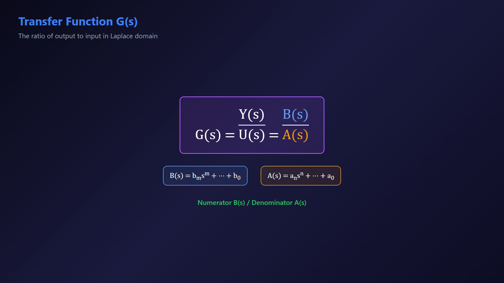
Read the formulas in the finite-dimensional LTI and zero-initial-state setting. The RC and RLC examples use the general transfer-function definition card; the motor uses the general LTI equation card. The integrator comparison uses the Laplace operator card. These are algebraic references, not physical circuit wiring or a completed motor diagram. Count transfer-function order after cancellation of common polynomial factors.
Apply the model to a parallel RC circuit; use the algebraic reference card.
Current balance:
$\displaystyle C\cdot y'\left(t\right) + \left(\frac{1}{R}\right)\cdot y\left(t\right) = u\left(t\right).$
Zero-state transform:
$\displaystyle \left(s\cdot C +\frac{ 1}{R}\right)\cdot Y\left(s\right) = U\left(s\right).$
RC impedance:
$\displaystyle G\left(s\right) = 1/\left(s\cdot C +\frac{ 1}{R}\right).$
This positive finite-RC model has reduced order one.
Narration transcript
Let us see an example. For an RC circuit with input current and output voltage, the differential equation is C times d y by d t plus one over R times y equals u. Applying the Laplace transform gives s C Y of s plus one over R times Y of s equals U of s. Solving for the ratio, G of s equals one over s C plus one over R. This is a first-order transfer function.
10. Derive the parallel RLC transfer function
Read the formulas in the finite-dimensional LTI and zero-initial-state setting. The RC and RLC examples use the general transfer-function definition card; the motor uses the general LTI equation card. The integrator comparison uses the Laplace operator card. These are algebraic references, not physical circuit wiring or a completed motor diagram. Count transfer-function order after cancellation of common polynomial factors.
Consider the parallel RLC current-input, voltage-output model.
Differentiated KCL:
$\displaystyle C\cdot y''\left(t\right) + \left(\frac{1}{R}\right)\cdot y'\left(t\right) + \left(\frac{1}{L}\right)\cdot y\left(t\right) = u'\left(t\right).$
RLC impedance:
$\displaystyle G\left(s\right) = s/\left(s²\cdot C +\frac{ s}{R }+\frac{ 1}{L}\right).$
For finite positive R, L and C this reduced transfer has order two.
Narration transcript
Now consider an RLC circuit. The differential equation is second order: C times d squared y by d t squared, plus one over R times d y by d t, plus one over L times y, equals d u by d t. The Laplace transform gives G of s equals s, divided by s squared C plus s over R plus one over L. This is a second-order transfer function.
11. Interpret the motor transfer blocks
Read the formulas in the finite-dimensional LTI and zero-initial-state setting. The RC and RLC examples use the general transfer-function definition card; the motor uses the general LTI equation card. The integrator comparison uses the Laplace operator card. These are algebraic references, not physical circuit wiring or a completed motor diagram. Count transfer-function order after cancellation of common polynomial factors.
Keep the electrical and mechanical motor couplings.
Read each component block within the complete coupled signal graph.
Use electrical factor 1/(L_a·s), fixed coupling K and mechanical factor 1/(J·s).
For the voltage-to-speed transfer, specify zero load torque and zero initial states.
Narration transcript
For the DC motor we studied earlier, the system has multiple loops. Each loop has its own transfer function block. The integrator one over L a s represents armature inductance, gain c phi F converts current to torque, and integrator one over J s represents the mechanical side. By combining these blocks, we can derive the complete motor transfer function.
12. Retain gains and replace integrators
Read the formulas in the finite-dimensional LTI and zero-initial-state setting. The RC and RLC examples use the general transfer-function definition card; the motor uses the general LTI equation card. The integrator comparison uses the Laplace operator card. These are algebraic references, not physical circuit wiring or a completed motor diagram. Count transfer-function order after cancellation of common polynomial factors.
Apply the transform to an otherwise correct signal graph.
Replace time integrators by their zero-state Laplace operators.
Integrator transfer:
$\displaystyle H\left(s\right) = 1/s.$
Preserve constant gains and every signed summing connection.
Use the Laplace operator card as an algebraic reference.
Narration transcript
Notice something important. We replaced the integrators in the time domain block diagram with their Laplace equivalents. An integrator in time becomes one over s in the Laplace domain. The gain blocks remain the same, and the overall structure is preserved. This gives us a clean transfer function representation.
13. Review the zero-state LTI model
Read the formulas in the finite-dimensional LTI and zero-initial-state setting. The RC and RLC examples use the general transfer-function definition card; the motor uses the general LTI equation card. The integrator comparison uses the Laplace operator card. These are algebraic references, not physical circuit wiring or a completed motor diagram. Count transfer-function order after cancellation of common polynomial factors.
Review the model.
A transfer function captures the selected LTI zero-state input-output channel.
Transfer definition:
$\displaystyle G\left(s\right) = Y\left(s\right)/U\left(s\right).$
Compare the parallel RC, parallel RLC and coupled motor examples.
Continue with impulse response and convolution.
Conclude the lesson.
Narration transcript
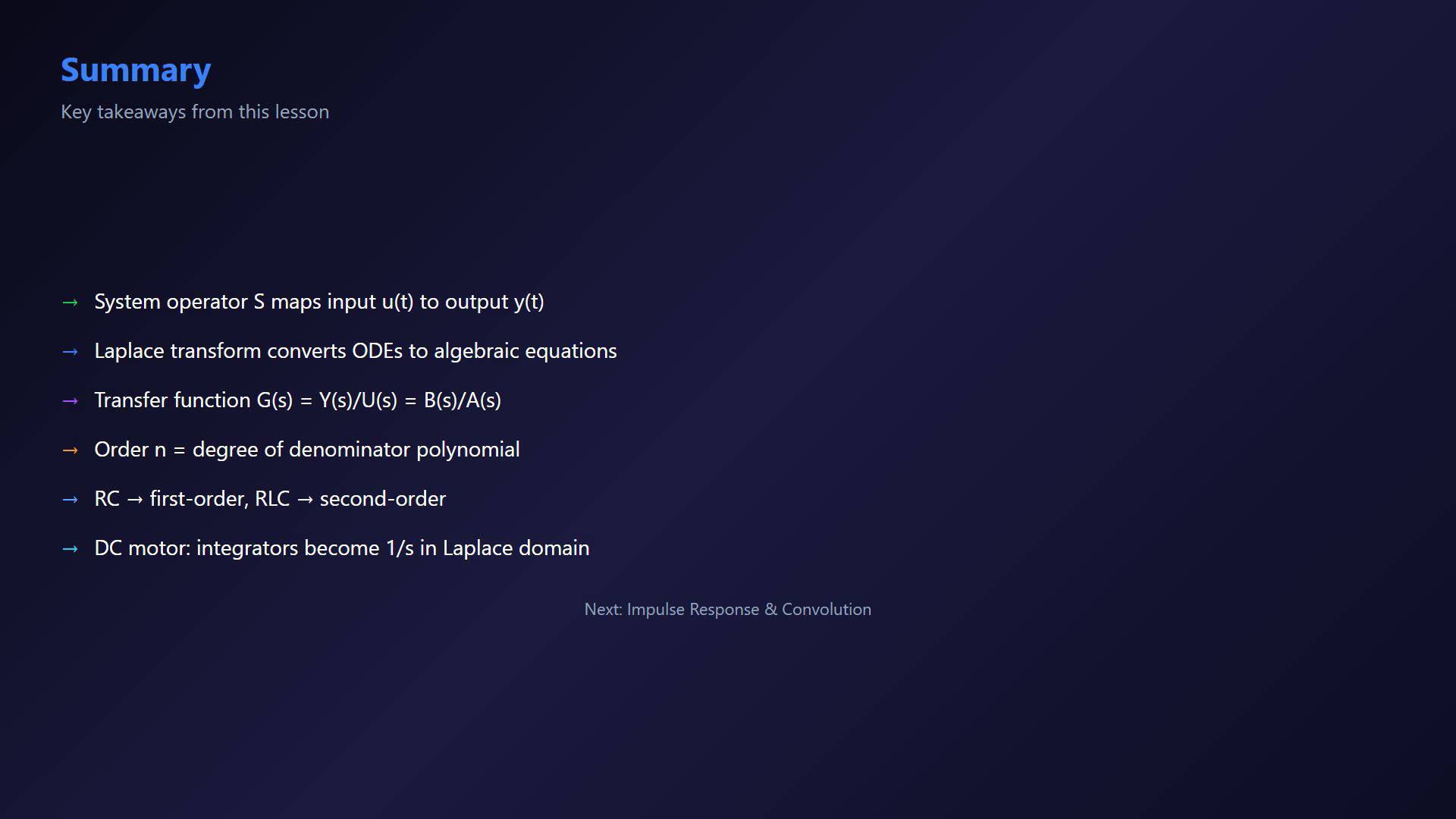
Excellent. In this lesson, we learned that the transfer function G of s captures the complete input-output behavior of a linear system. It is the ratio of output to input in the Laplace domain. We saw examples for RC, RLC, and DC motor systems. In the next lesson, we explore impulse response and convolution. See you there.