Electromagnetic Theory · Divergence — Worked Examples
#28 Cartesian divergence and the singular inverse-square radial field
Compute Cartesian divergence, apply the spherical radial formula, and distinguish zero local divergence from nonzero flux enclosing a point source.
Question
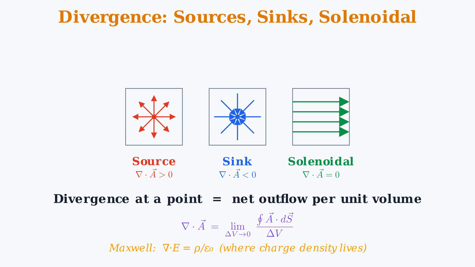
Find the divergence of two vector fields. In the writing lines, D denotes the scalar divergence of A, and D_E denotes the scalar divergence of the electric field E. Cartesian A=(A_x,A_y,A_z) and spherical A=(A_r,A_θ,A_φ) are ordered components in the corresponding local orthonormal unit-vector basis. They are not a scalar sum of components. The source recap abbreviates the three Cartesian terms verbally; the full field definition and original graphic retain their respective unit-vector directions. For a continuously differentiable vector field, divergence at a point is the limit of net outward flux through a shrinking closed surface divided by its enclosed volume. A positive value gives a local source tendency and a negative value a local sink tendency. This smooth distributed behavior does not by itself imply a singular point source or the creation of fluid mass. For a velocity field, zero divergence throughout a region is the local volume-preserving condition associated with incompressible flow. Zero divergence at one point alone does not establish that a whole field is solenoidal or that every finite surrounding volume has exactly zero flux. For a smooth field with zero divergence throughout a closed volume, total inward and outward fluxes balance. Drawn field lines are a qualitative picture of flux, not countable physical objects; the number of arrows is not a numerical divergence measurement. Use Cartesian coordinates (x,y,z), cylindrical (ρ,φ,z) away from ρ=0, and spherical (r,θ,φ) away from r=0 and the polar coordinate axes. Spherical θ is measured from +z and φ is azimuth from +x toward +y; angular derivatives use radians. Component formulas refer to the local orthonormal basis. In Cartesian coordinates, D=∂A_x/∂x+∂A_y/∂y+∂A_z/∂z. In cylindrical coordinates, D=(1/ρ)∂(ρA_ρ)/∂ρ+(1/ρ)∂A_φ/∂φ+∂A_z/∂z. In spherical coordinates, D=(1/r²)∂(r²A_r)/∂r+(1/(r sinθ))∂(sinθ A_θ)/∂θ+(1/(r sinθ))∂A_φ/∂φ. In the three spherical contribution lines, R,T,F denote these radial, polar and azimuthal scalar terms; their sum is D. The denominator r sinθ is the entire product. Keep ρ, r² and sinθ inside the indicated derivatives; they reflect the changing physical volume associated with equal coordinate increments. Example 1 has Cartesian components (x²y,y²z,z²x) at P=(1,2,3). Differentiate each component only with respect to its matching coordinate, holding the others fixed. The three partials are 2xy,2yz,2zx. Their values at P are 4, 12, 6, giving D(P)=22. The result is a scalar, not the vector(4,12,6), and not the sum of the original field components. More generally D(x,y,z)=2xy+2yz+2zx, so the result depends on position and different points can sometimes have the same value. Positive 22 means a sufficiently small volume around P has positive net outward flux. For a symmetric cube centered at P, direct integration of this polynomial field gives flux 22 times the cube's volume. Example 2 is the outward radial field A=(1/r²)e_r for r>0. Its angular components vanish, leaving D=(1/r²)∂(r²A_r)/∂r. Simplify inside the derivative: r²A_r=1, whose derivative is zero. Therefore D=0 for r>0. Taking only the derivative of 1/r² and forgetting the inner r² would be incorrect. In Cartesian form the same field is (x,y,z)/(x²+y²+z²)^(3/2), defined away from the origin, which provides an independent check including points on a spherical coordinate axis. The field is undefined at the origin, so do not assign its classical divergence there or apply the smooth divergence theorem to a volume containing the origin without accounting for the singularity. On an outward-oriented sphere centered at the origin, A has normal component 1/r² and the area is 4πr², so the total flux is 4π for every positive radius. More generally any suitable closed surface enclosing the origin once has the same flux; a closed surface excluding it has zero flux. In the distributional description the divergence is 4π times the three-dimensional delta distribution at the origin. This does not contradict the pointwise zero divergence for r>0. It explains the source concentration mentioned by the original video. For a point charge q in vacuum, the electric field is q/(4π ε_0) times this radial field, so its enclosed flux is q/ε_0 and D_E=ρ_q/ε_0, with ρ_q the charge density. Charge density here is distinct from the cylindrical radius ρ. The sign and physical coefficient depend on the example: a positive charge gives an outward electric field; Newtonian gravity of a positive point mass is inward, with a negative radial coefficient. The source comparison concerns inverse-square radial dependence, not identical force direction or omitted physical constants. The next operator, curl, returns a vector and is a separate calculation.
Written solution and narration transcript(shows the full solution)
Below are all the lines written in the notebook together with the full narration transcript.
1. Sources, sinks and divergence
Divergence is a scalar. Include each coordinate scale factor inside its required derivative and keep the inverse-square result restricted to points away from the singular origin. Divergence of a vector fieldGradient takes a scalar field to a vector field.Now consider divergence.Divergence takes a vector field to a scalar field.Write D for the scalar divergence of A at each point.It is the limit of outward flux divided by the enclosed small volume.A fluid velocity field provides an intuitive example.Positive divergence describes local net outflow.Negative divergence describes local net inflow.Zero divergence throughout a region defines a solenoidal field.The same operator appears in electromagnetism.Electric-field divergence:This is the differential form of Gauss’s law.Divergence locates distributed sources and sinks.Narration transcript
Hello friends, welcome back. In the last worked example we computed the gradient — the operator that takes a scalar field and gives back a vector. Today we meet a different beast: the divergence. The divergence takes a vector field and returns a scalar. So if A is a vector at every point of space, nabla dot A is a number at every point. Geometrically, the divergence at a point measures the net outflow of the field from that point, per unit volume. Think of A as the velocity of a fluid. If divergence is positive, more fluid leaves a tiny box around the point than enters — there is a source inside. If divergence is negative, more fluid enters than leaves — there is a sink. If divergence is zero, whatever flows in also flows out — the field is incompressible, or as we say in electromagnetics, solenoidal. This is more than fluid dynamics. In electrostatics, the divergence of the electric field at a point equals the charge density there, divided by epsilon zero. That is one of Maxwell's equations. So divergence is a way to ask: where are the sources of the field?
2. Three divergence formulas
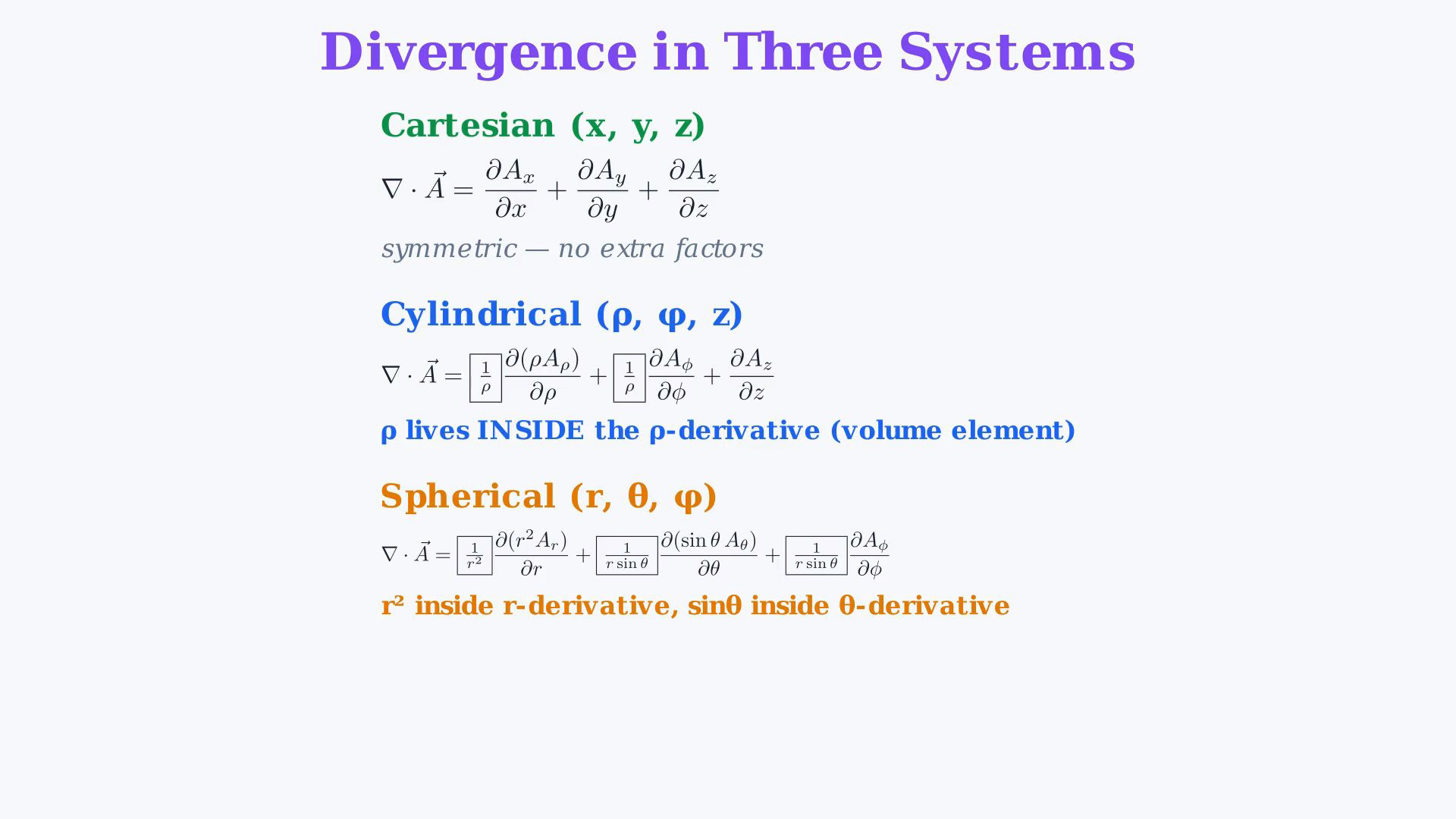
Divergence is a scalar. Include each coordinate scale factor inside its required derivative and keep the inverse-square result restricted to points away from the singular origin. Volume scale factors depend on the coordinate system.Cartesian:Differentiate each component with respect to its matching coordinate.Cylindrical:Keep ρ inside the radial derivative.Spherical radial contribution:Spherical polar contribution:Spherical azimuthal contribution:Equal coordinate increments can enclose different physical volumes.A fixed azimuthal sweep spans a longer arc farther from the axis.Divergence measures net flux per unit volume.Apply the formulas to two fields.Narration transcript
The divergence formula has the same shape in every coordinate system, but with different factors that account for how the volume element changes. In Cartesian: nabla dot A equals partial Ax over partial x, plus partial Ay over partial y, plus partial Az over partial z. Three partial derivatives, no extra factors, perfectly symmetric. In cylindrical: nabla dot A equals one over rho times partial of rho times A-rho with respect to rho, plus one over rho times partial of A-phi with respect to phi, plus partial of A-z with respect to z. Notice the rho appears INSIDE the rho derivative — that is the volume element distortion. In spherical: the radial term is one over r squared times partial of r squared times A-r with respect to r. The theta term is one over r sine theta times partial of sine theta times A-theta with respect to theta. The phi term is one over r sine theta times partial of A-phi with respect to phi. The deeper why: in non-Cartesian systems, the volume of a tiny box depends on where it is. Near the cylindrical axis a small phi sweep covers little arc; far away it covers a lot. The divergence asks for net flux per VOLUME, so the formula must include those geometric factors. We will see them in action right now.
3. Cartesian worked example
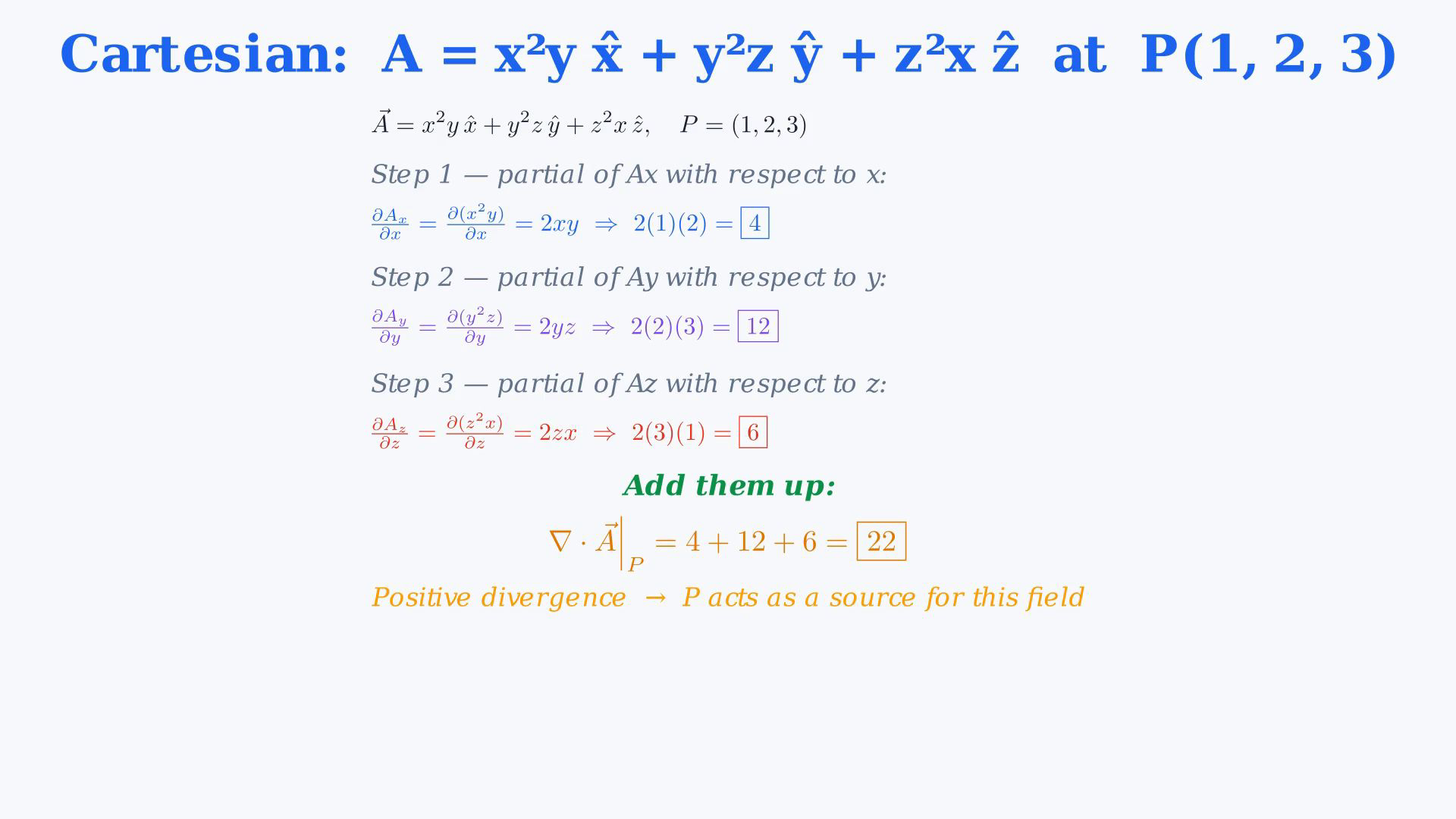
Divergence is a scalar. Include each coordinate scale factor inside its required derivative and keep the inverse-square result restricted to points away from the singular origin. Worked example 1: CartesianCartesian vector components:Given point:Find the scalar divergence at P.Use three matching component derivatives.Step 1: the x component.First component:Hold y fixed:At P:Step 2: the y component.Second component:Hold z fixed:At P:Step 3: the z component.Third component:Hold x fixed:At P:Add the derivatives:The divergence is positive at P.A sufficiently small surrounding volume has positive net outward flux.This is a local source tendency of the smooth field.The divergence depends on position.Narration transcript
Worked example one — Cartesian. Take A equal to x squared y x-hat, plus y squared z y-hat, plus z squared x z-hat. Our point is P equals one, two, three. We want the divergence at P. Three steps, one for each component. Step one. Take partial of Ax with respect to x, where Ax equals x squared y. The y is a constant when we differentiate with respect to x, so we get two x y. At P, that is two times one times two, which equals four. Step two. Take partial of Ay with respect to y, where Ay equals y squared z. Now z is the constant; the derivative is two y z. At P, that is two times two times three, which equals twelve. Step three. Take partial of Az with respect to z, where Az equals z squared x. With x constant, the derivative is two z x. At P, that is two times three times one, which equals six. Add the three: nabla dot A at P equals four plus twelve plus six, which is twenty-two. Interpretation: the divergence is positive at P. If A were the velocity of a fluid, more fluid would be leaving a tiny box around P than entering. P behaves like a source for this field. If we picked a different point, the answer would change — divergence is a local quantity.
4. Inverse-square radial field
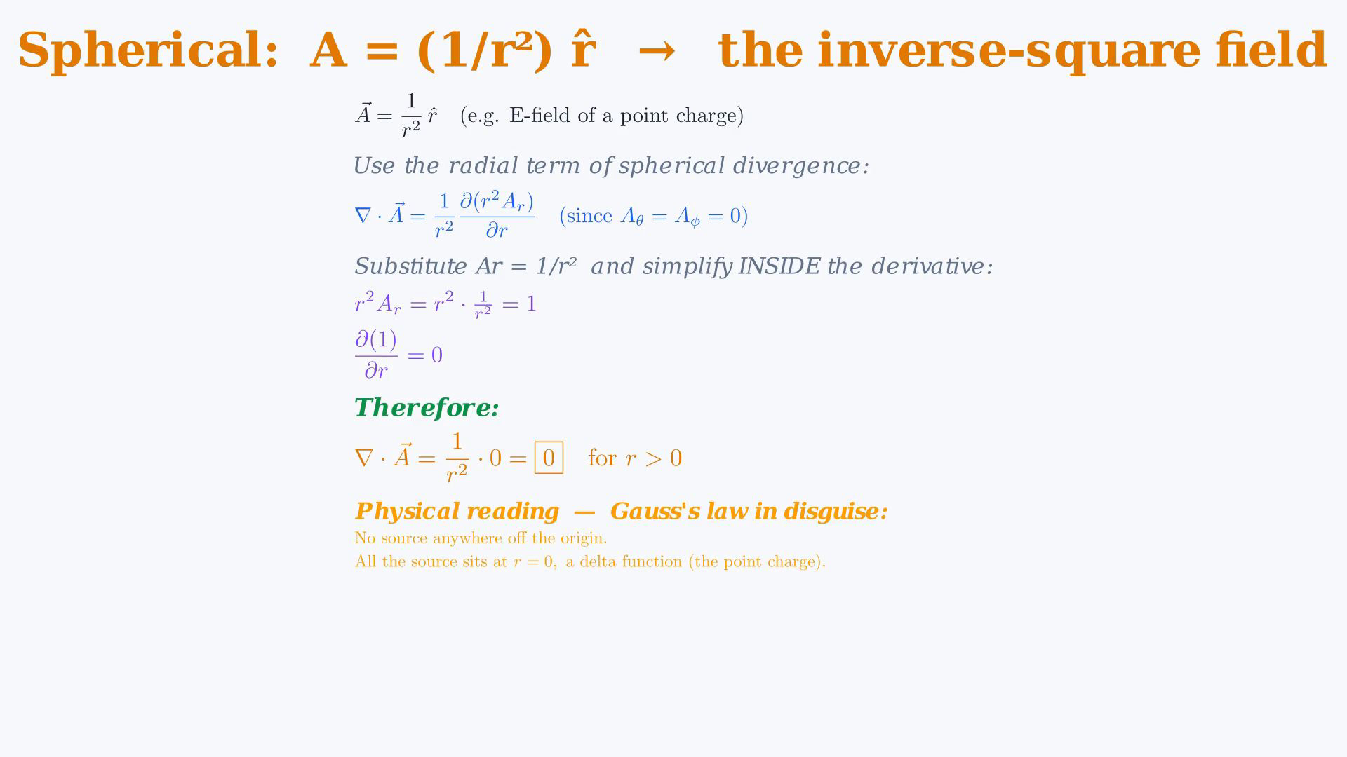
Divergence is a scalar. Include each coordinate scale factor inside its required derivative and keep the inverse-square result restricted to points away from the singular origin. Worked example 2: a radial fieldSpherical vector components:The magnitude follows an inverse-square law away from the origin.A point charge has this radial dependence, with a physical coefficient.Point-mass gravity has the same radial dependence with an inward sign.A constant multiple retains the inverse-square radial form.Find the divergence away from the origin.Only the radial component contributes.Radial divergence:Substitute:Inside the derivative:Derivative of the constant:For positive r:Interpret the result.Classical divergence is zero everywhere off the origin.Any closed volume excluding the origin has zero net flux.There are no distributed sources away from the origin.The origin is singular and requires a separate source description.Closed surfaces enclosing the origin carry the same total outward flux.This distinction is central to Gauss’s law.Narration transcript
Worked example two — spherical, and this is the example that every electromagnetics student should keep in their pocket. Take A equal to one over r squared, in the r-hat direction. This is the famous inverse-square radial field. The electric field outside a point charge looks like this. The gravitational field outside a point mass looks like this. Anything spherically symmetric and falling off as one over r squared looks like this. Find the divergence. The spherical formula has three terms, but A only has an r-hat component, so only the r-term matters. Nabla dot A equals one over r squared, times the partial with respect to r, of r squared times A-r. Plug in A-r equals one over r squared. The expression inside the derivative becomes r squared times one over r squared, which is just one. The derivative of one with respect to r is zero. So nabla dot A equals one over r squared, times zero, which is zero — for every r greater than zero. Stop and feel that. Everywhere in space, except at the origin, this radial inverse-square field has zero divergence. If you draw a tiny box anywhere off the origin, the same number of field lines enter as leave. There are no sources out there. All the source is concentrated at the origin, where the formula breaks down. That is the mathematical heart of Gauss's law: a point charge produces a one over r squared field whose divergence is zero everywhere except where the charge sits, and integrating around the charge always gives the same total outflow, no matter how big or small your surface. This is going to come back many times in this course.
5. Divergence recap
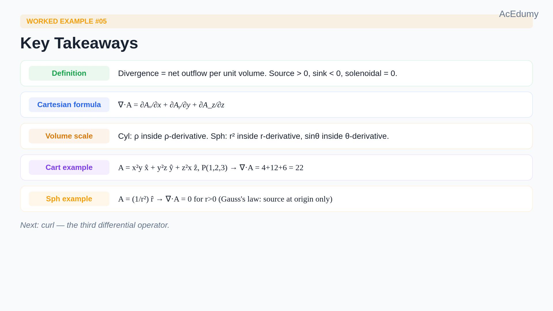
Divergence is a scalar. Include each coordinate scale factor inside its required derivative and keep the inverse-square result restricted to points away from the singular origin. Divergence recapVector field to scalar field: local net outflow per volume.Use the sign to distinguish source, sink and zero divergence.Keep the complete coordinate formulas.Cartesian:Cylindrical:Spherical:Keep radial factors inside the radial derivatives.Two worked results.Cartesian result at P:Inverse-square radial field for positive r:Next: curl of a vector field.End of the worked examples.Narration transcript
Quick recap. Divergence turns a vector field into a scalar; it measures net outflow per unit volume. Positive means a source, negative means a sink, zero means solenoidal. The formulas. Cartesian: partial Ax over x, plus partial Ay over y, plus partial Az over z. Cylindrical: one over rho times partial of rho A-rho with respect to rho, plus one over rho times partial A-phi with respect to phi, plus partial Az with respect to z. Spherical: one over r squared times partial of r squared A-r with respect to r, plus one over r sine theta times partial of sine theta A-theta with respect to theta, plus one over r sine theta times partial A-phi with respect to phi. The volume scale factors live INSIDE the derivatives for the radial terms — that is the part students miss most. Two answers. Cartesian, A equals x squared y plus y squared z plus z squared x at P one two three: divergence equals twenty-two. Spherical, A equals one over r squared times r-hat: divergence equals zero, anywhere away from the origin. Next worked example: the curl, the third differential operator. See you then.
Source video: Electromagnetic Theory (v2) #28 | Problem Solving #05: Divergence of a Vector Field (8:24)