#11 Potential difference, point and continuous-charge potentials, superposition, E = −∇V, and conservative electrostatic fields

Below are all the lines written in the notebook together with the full narration transcript.

1. 1. Move from Gauss's law to scalar potential

   

   Last time, we defined the electric flux density D and derived Gauss's law — the first of Maxwell's equations.

   With symmetry, Gauss's law lets us find D in just a few lines of algebra.

   Today, we introduce the electric potential V — a scalar quantity that provides yet another way to find the electric field.

   We'll derive the E-V relationship, which is the second Maxwell equation for static fields, and show why working with a scalar is often much easier than working with vectors.

   Narration transcript

   Last time, we defined the electric flux density D and derived Gauss's law — the first of Maxwell's equations. With symmetry, Gauss's law lets us find D in just a few lines of algebra. Today, we introduce the electric potential V — a scalar quantity that provides yet another way to find the electric field. We'll derive the E-V relationship, which is the second Maxwell equation for static fields, and show why working with a scalar is often much easier than working with vectors.

2. 2. Define potential difference and point charge

   

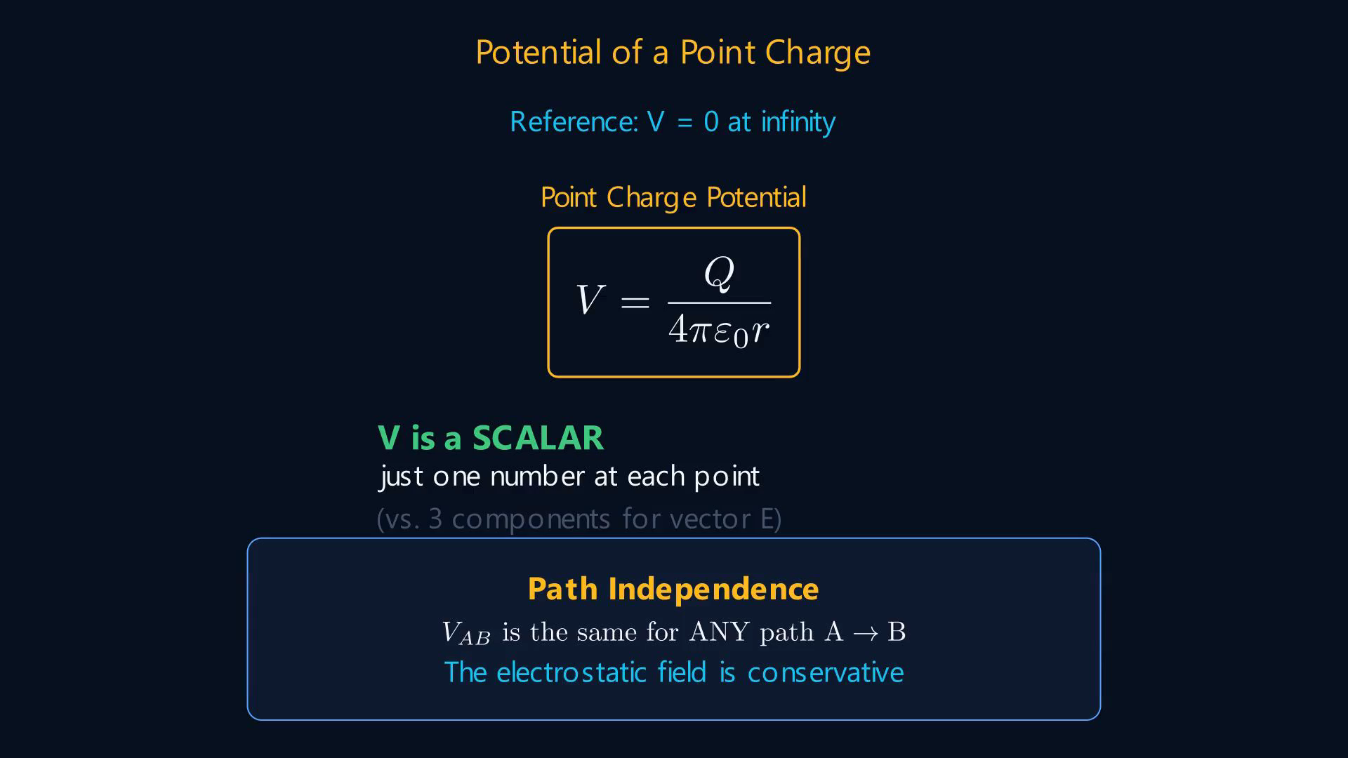
   Suppose we move a point charge Q from point A to point B in an electric field E.

   External work: W_ext = −Q∫ₐᵇE·dl.

   Potential difference: V_AB = V_B − V_A = −∫ₐᵇE·dl.

   This quantity V_AB is measured in volts — joules per coulomb.

   For a point charge Q at the origin, the E field is radial.

   With V(∞)=0, a point charge has V = Q/(4πε₀r).

   This is a crucial result.

   Unlike the vector E which has three components, V is a scalar — just one number at each point in space.

   And the potential difference V_AB is independent of the path taken between A and B.

   The electrostatic field is conservative.

   Narration transcript

   Suppose we move a point charge Q from point A to point B in an electric field E. The work done by an external agent against the field is: W equals minus Q times the line integral of E dot d-l from A to B. Dividing by Q gives the potential difference between A and B: V-A-B equals minus the integral of E dot d-l from A to B. This quantity V-A-B is measured in volts — joules per coulomb. For a point charge Q at the origin, the E field is radial. Taking the reference at infinity where V equals zero, the potential at distance r is: V equals Q over four pi epsilon-zero r. This is a crucial result. Unlike the vector E which has three components, V is a scalar — just one number at each point in space. And the potential difference V-A-B is independent of the path taken between A and B. The electrostatic field is conservative.

3. 3. Add point and continuous-charge potentials

   

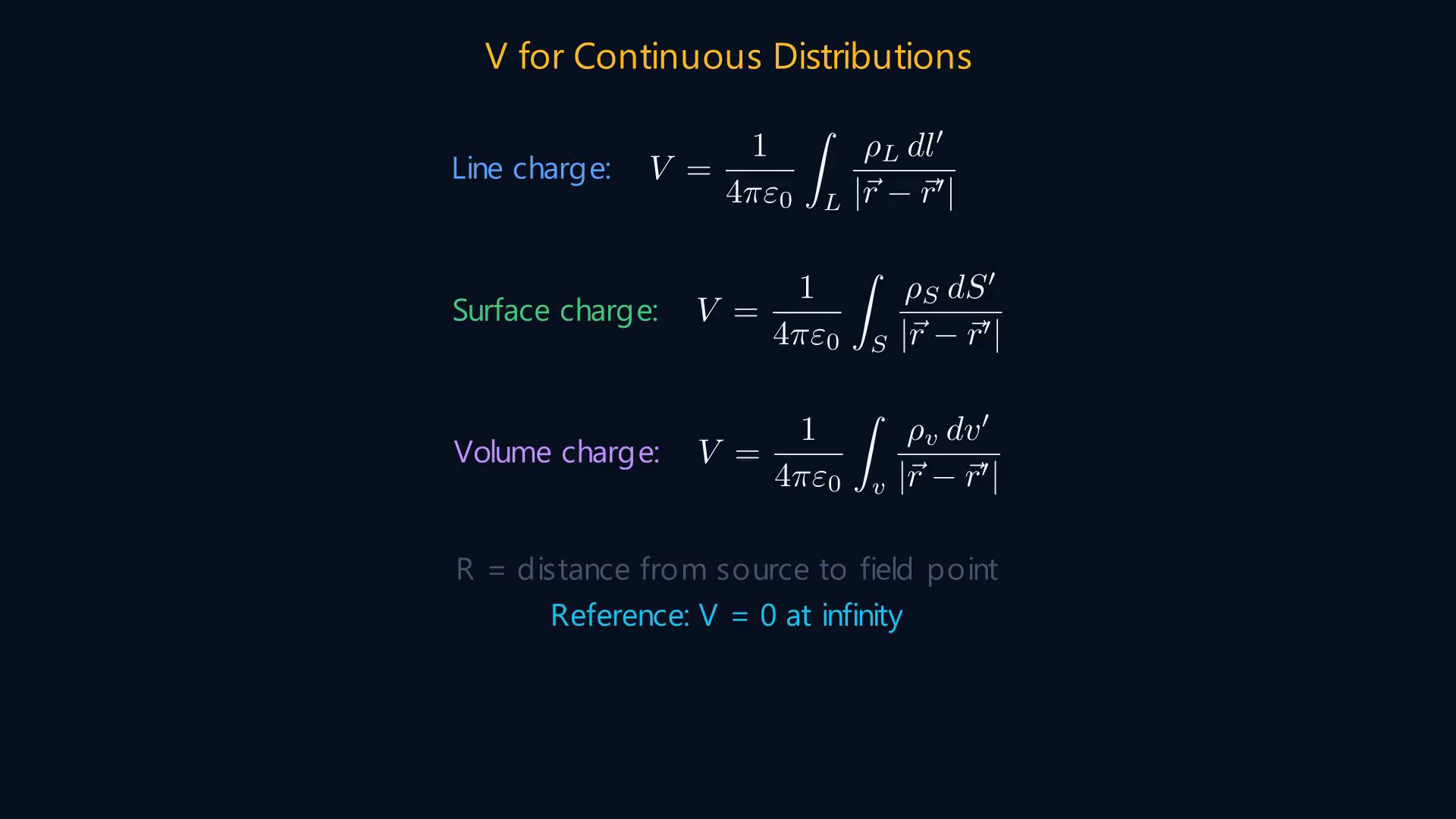
   Just as E obeys superposition, so does V.

   For N point charges, V(r) = ΣₖQₖ/[4πε₀|r − rₖ|].

   Notice the enormous advantage: we're summing scalars, not vectors.

   No need to decompose into components and add separately.

   For continuous charge distributions, we replace the sum with an integral.

   Line charge: V = ∫ₗρ_L dl/(4πε₀R).

   Surface charge: V = ∫ₛρ_S dS/(4πε₀R).

   Volume charge: V = ∫ᵥρ_v dv/(4πε₀R).

   In each case, R is the distance from the source element to the field point.

   The reference point where V equals zero is taken at infinity.

   Narration transcript

   Just as E obeys superposition, so does V. For n point charges Q-one through Q-n at positions r-one through r-n, the potential at any point r is: V equals the sum of Q-k over four pi epsilon-zero times the magnitude of r minus r-k. Notice the enormous advantage: we're summing scalars, not vectors. No need to decompose into components and add separately. For continuous charge distributions, we replace the sum with an integral. For a line charge: V equals the integral of rho-L d-l over four pi epsilon-zero R. For a surface charge: V equals the integral of rho-S d-S over four pi epsilon-zero R. For a volume charge: V equals the integral of rho-v d-v over four pi epsilon-zero R. In each case, R is the distance from the source element to the field point. The reference point where V equals zero is taken at infinity.

4. 4. Derive E = −∇V and conservativeness

   

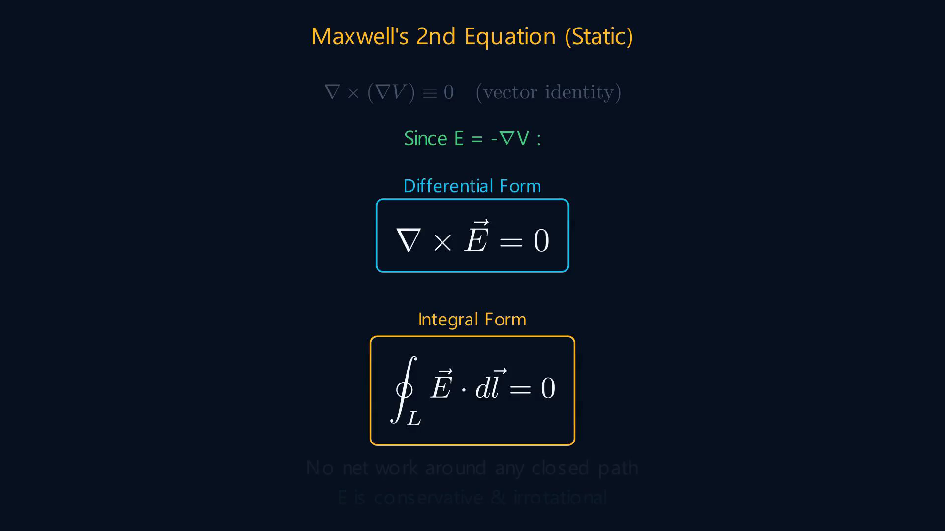
   Potential difference is V_AB = −∫ₐᵇE·dl.

   The total differential is dV = (∂V/∂x)dx + (∂V/∂y)dy + (∂V/∂z)dz.

   Comparing them gives E = −grad V.

   In other words, E = −∇V.

   This is tremendously useful.

   If we know V — a single scalar function — we can find all three components of E by taking partial derivatives.

   E points from higher potential to lower potential, and its magnitude is greatest where V changes most rapidly.

   Since every gradient is irrotational, ∇×E = 0.

   This is Maxwell's second equation for static fields.

   Integral form: ∮E·dl = 0.

   Physically, no net work is done in moving a charge around any closed path in an electrostatic field.

   This confirms that the electrostatic field is conservative and irrotational.

   Narration transcript

   We defined the potential as V equals minus the integral of E dot d-l. But from multivariable calculus, the total differential d-V equals partial V partial x d-x plus partial V partial y d-y plus partial V partial z d-z. Comparing these two expressions, we find: E equals minus the gradient of V. In other words, E equals minus nabla V. This is tremendously useful. If we know V — a single scalar function — we can find all three components of E by taking partial derivatives. E points from higher potential to lower potential, and its magnitude is greatest where V changes most rapidly. Now, since the curl of any gradient is identically zero, we get: nabla cross E equals zero. This is Maxwell's second equation for static fields. Its integral form is: the closed line integral of E dot d-l equals zero. Physically, no net work is done in moving a charge around any closed path in an electrostatic field. This confirms that the electrostatic field is conservative and irrotational.

5. 5. Calculate E and work in spherical coordinates

   

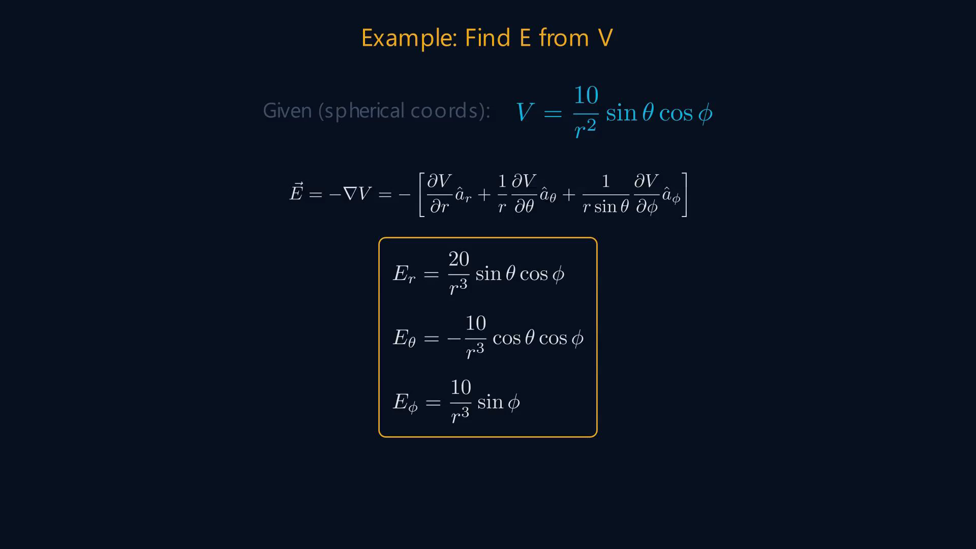
   Let's see how the E-V relationship simplifies calculations.

   Given V = (10/r²)sinθ cosφ, find E and the work required to move a charge.

   First, E = −∇V.

   Spherical gradient:

   $\displaystyle ∇V =\frac{ e_{r}\partial V}{\partial r }+\frac{ e_{\theta }\left(\frac{1}{r}\right)\partial V}{\partial \theta }+ e_{\varphi }\left[\frac{1}{r \sin \theta }\right]\partial V/\partial \varphi .$

   $\displaystyle E_{r} = \left(20/r³\right)\sin \theta \cos \varphi , E_{\theta } = -\left(10/r³\right)\cos \theta \cos \varphi , E_{\varphi } = \left(10/r³\right)\sin \varphi .$

   $\displaystyle q = 10 \mu C; A=\left(1,30^{\circ},120^{\circ}\right), B=\left(4,90^{\circ},60^{\circ}\right).$

   W_ext = qV_AB = q(V_B − V_A).

   Just plug in the coordinates.

   Correct intermediate values: V_A = −2.5 V and V_B = 10/32 = 0.3125 V.

   W_ext = 10 μC × 2.8125 V = 28.125 μJ.

   No line integrals needed — that's the power of working with the scalar potential.

   Narration transcript

   Let's see how the E-V relationship simplifies calculations. Given the potential V equals ten over r-squared times sine theta cosine phi in spherical coordinates, find E and calculate the work done in moving a charge. First, E equals minus nabla V. In spherical coordinates, the gradient has three terms: partial with respect to r, one over r partial with respect to theta, and one over r sine theta partial with respect to phi. Taking each partial derivative, we get: E-r equals twenty over r-cubed sine theta cosine phi, E-theta equals minus ten over r-cubed cosine theta cosine phi, and E-phi equals ten over r-cubed sine phi. Now for the work: moving a ten micro-coulomb charge from point A at r equals one, theta equals thirty degrees, phi equals one-twenty degrees, to point B at r equals four, theta equals ninety degrees, phi equals sixty degrees. Method two is much easier: W equals Q times V-A-B, which is Q times V-B minus V-A. Just plug in the coordinates. V at A is minus five, V at B is ten over thirty-two. So W equals ten micro-coulombs times the difference, giving twenty-eight point one-two-five micro-joules. No line integrals needed — that's the power of working with the scalar potential.

6. 6. Review the potential–field relationship

   

   Let's recap today's key ideas.

   V_AB = −∫ₐᵇE·dl; the potential difference is path-independent.

   For a point charge, V = Q/(4πε₀r).

   Potential obeys superposition — sum scalars, not vectors.

   E = −∇V; obtain the vector field from a scalar function.

   This is Maxwell's second static equation in differential form.

   Integral form: ∮E·dl = 0.

   Next time, we'll explore the electric dipole and energy stored in electrostatic fields.

   Narration transcript

   Let's recap today's key ideas. V-A-B equals minus the integral of E dot d-l — the potential difference is path-independent. For a point charge: V equals Q over four pi epsilon-zero r. Potential obeys superposition — sum scalars, not vectors. E equals minus nabla V — find the vector field from a scalar function. This is Maxwell's second static equation in differential form. The integral form is: the closed line integral of E dot d-l equals zero. Next time, we'll explore the electric dipole and energy stored in electrostatic fields.

Source video: Electromagnetic Theory (v2) #11 Electric Potential (V) & E-V Relationship (6:45)