Circuit Theory 2 · Frequency response and decibels
#20 Stable causal sinusoidal response, RC low-pass magnitude and phase, and amplitude versus power decibels
Read the RC gain, phase and corner frequency, with clear π/ω formulas and separate amplitude and power decibel assumptions.
Question
Use an ideal real linear time-invariant circuit, constant positive R and C, a voltage input and unloaded capacitor-voltage output relative to the same reference. H(s)=1/(τs+1), τ=RC>0 is the initially relaxed transfer function. Its causal region Re(s)>−1/τ contains the imaginary axis; only under the corresponding existence/stability conditions may H(jω) be read as frequency response with settling sinusoidal steady state. An unstable circuit or a pole on the excited imaginary-axis frequency may not settle. For input A cos(ωt), the steady-state part is A|H(jω)|cos(ωt+φ), φ=arg H(jω); y_ss excludes the switched-on transient. Phase is undefined when the output gain is zero, and the unchanged-frequency statement concerns linear time-invariant response, not nonlinear frequency conversion. Phase advance or lag for one sinusoid is not a frequency-independent delay of a general waveform. For the RC circuit H(jω)=1/(1+jωτ), magnitude1/sqrt(1+(ωτ)^2), and φ=−arctan(ωτ). Square the entire dimensionless product ωτ; the phase formula returns radians unless converted to degrees. For ω>0 the phase is negative, tending from0 to−90degrees. At ω_c=1/τ, magnitude1/sqrt(2), phase−45degrees; f_c=1/(2πτ) in hertz, while ω=2πf is radians per second. DC voltage gain is one; high-frequency magnitude tends to zero. The approximation H≈1 applies well below the corner, not throughout the entire region below it. For a positive dimensionless amplitude ratio r, define G_A(r)=20log10(r); use consistent peak or RMS conventions. Thus G_A(1)=0, G_A(1/sqrt(2))=−10log10(2)≈−3.0103, G_A(.1)=−20, G_A(10)=20 decibels. Separately the frequency curve is G(ω)=20log10|H(jω)|=−10log10(1+(ωτ)^2). For positive real power ratios use G_P=10log10(P2/P1). Equal positive resistances permit identifying the voltage-amplitude result with power gain; for unequal resistances, P2/P1=(V2/V1)^2 R1/R2 using RMS voltages. For current ratios the resistance factor is R2/R1. Do not infer half power from an amplitude ratio alone, especially for a reactive capacitor output with no resistive load. These qualifications do not change the definition of amplitude gain in decibels. Arguments of logarithms must be positive and dimensionless; zero gain has a limiting value of minus infinity decibels. The exact RC logarithmic slope is −20(ωτ)^2/(1+(ωτ)^2) dB per decade: −10 at the corner, tending to−20 only far above it. Before/after-corner narration is an asymptotic simplification, not an exact plateau or immediate exact slope. All nine original final frames were individually inspected. The Bode raster's numeric y-tick locations disagree with its plotted scale, so that role uses the same final's readable summary card. The decibel table calls the corner half power without impedance conditions, so that role uses the same final's traps card and the notebook states those conditions. No source video or new graphic was generated. The retained RC port diagram has minor capacitor/output-label overlap but an unambiguous connected topology; the phase plot is qualitative near its endpoint ticks. The sinusoid illustration omits a labelled zero-voltage baseline, so do not infer a DC offset from its panel coordinate placement. Original one-line fractions, omega/tau text and graph-label typography remain manual visual/teaching-QA caveats. Notebook formulas use the existing common renderer, with full denominators, Greek symbols and explicit assumptions. The original source say, all nine MP3s and all45 aligned cue boundaries remain unchanged. Full cached-large ASR recognized the numeric magnitudes, logarithm bases, pi conversion and negative phase signs; abbreviation omega-T in one passage remains an ASR tokenization observation, not evidence of wrong source speech. No alignment overrides, prompts or threshold changes. This is an unpublished draft, not full human listening, complete motion QA or publication approval.
Written solution and narration transcript(shows the full solution)
Below are all the lines written in the notebook together with the full narration transcript.
1. Evaluate the stable causal transfer function on the imaginary axis
Reference from the existing video. The decibel-table and Bode-plot roles use readable traps and summary cards from the same final; full formulas and the required conditions are stated in the notebook. For the chosen initially relaxed LTI circuit:Keep the same chosen input-output map.Now ask how each sinusoidal frequency is changed by a stable causal system.When the imaginary axis belongs to the transform region, evaluate there:Narration transcript
In the previous lesson, the transfer function was our zero-state map: Y of s equals X of s times H of s. Now we use that same map in a more practical way. Instead of asking for every possible time waveform, we ask how the circuit treats each sinusoidal frequency. The move is beautifully small: take H of s and evaluate it on the imaginary axis, by setting s equal to j omega.
2. Read frequency-dependent gain and phase
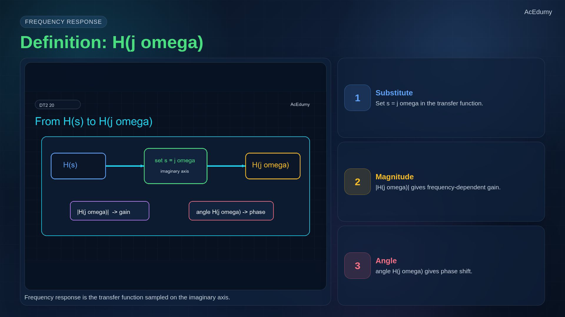
Reference from the existing video. The decibel-table and Bode-plot roles use readable traps and summary cards from the same final; full formulas and the required conditions are stated in the notebook. For a stable causal LTI circuit, its frequency response is the transfer function evaluated on the imaginary axis.At each angular frequency it has a complex gain.Its magnitude gives amplitude gain; its argument gives the phase shift.A phase lead or lag of one sinusoid is not automatically a frequency-independent time delay.Narration transcript
Frequency response is H of j omega. It is a complex number for every angular frequency omega. The magnitude tells us the gain at that frequency, and the angle tells us the phase shift. So the circuit becomes a frequency-by-frequency filter: some frequencies pass almost unchanged, some are attenuated, and each one can be delayed or advanced in phase.
3. Separate steady state from the transient
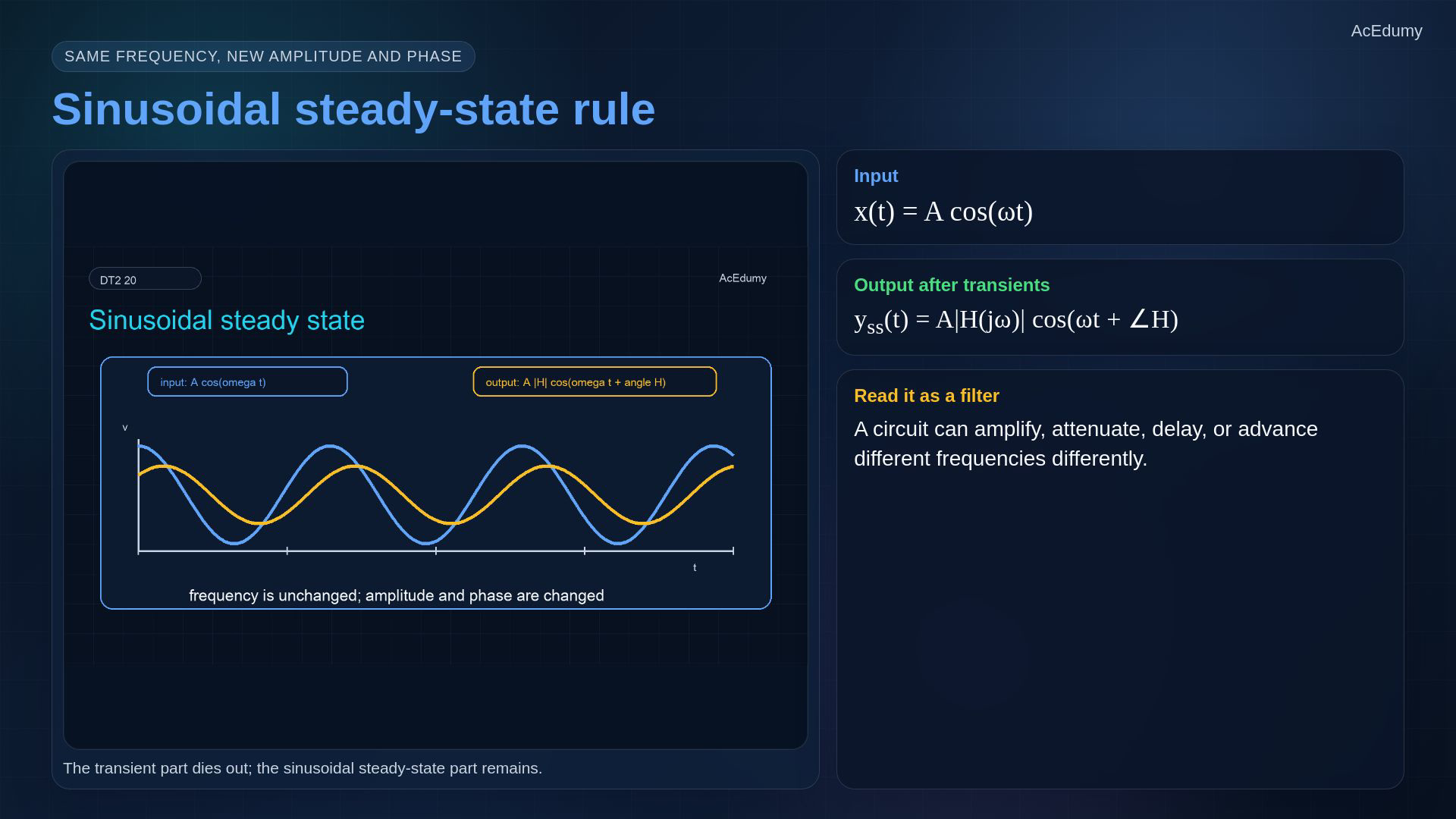
Reference from the existing video. The decibel-table and Bode-plot roles use readable traps and summary cards from the same final; full formulas and the required conditions are stated in the notebook. Use a real stable LTI circuit and wait for the transient to decay.For sinusoidal input, the steady-state output is:The steady-state frequency is unchanged.The gain and phase change; φ denotes the argument of the frequency response.This rule gives the steady-state part, not the complete switched-on waveform.Narration transcript
Here is the key steady-state rule. If the input is A cosine omega t, then after transients die out, the output is A times the magnitude of H of j omega, cosine of omega t plus the angle of H of j omega. The frequency stays the same. Only the amplitude and phase change. That is why frequency response is so powerful for sinusoidal analysis.
4. Apply the RC low-pass transfer function
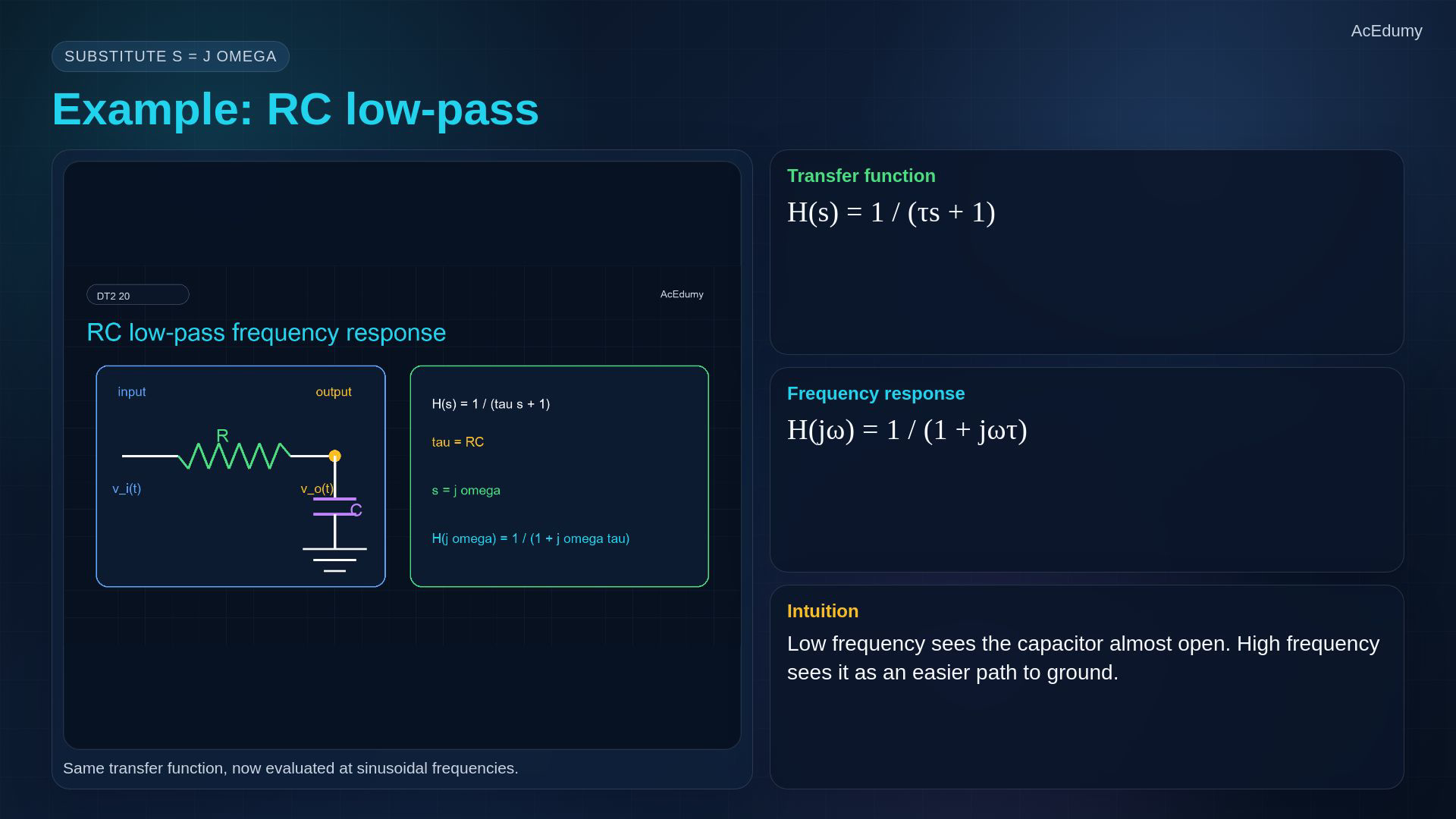
Reference from the existing video. The decibel-table and Bode-plot roles use readable traps and summary cards from the same final; full formulas and the required conditions are stated in the notebook. For the RC voltage low-pass with positive constant R and C:Its stable causal transform region contains the imaginary axis:The frequency response is:Well below the corner, the dimensionless product is small:Well above the corner, the voltage gain is small; this assumes the same input amplitude.Narration transcript
Use the same RC low-pass transfer function from last time: H of s equals one over tau s plus one, where tau equals R C. Frequency response means substitute s equals j omega. So H of j omega equals one over one plus j omega tau. At low frequency, omega tau is small, and the denominator is close to one. At high frequency, omega tau is large, and the output becomes small.
5. Read the complete magnitude and lag formulas
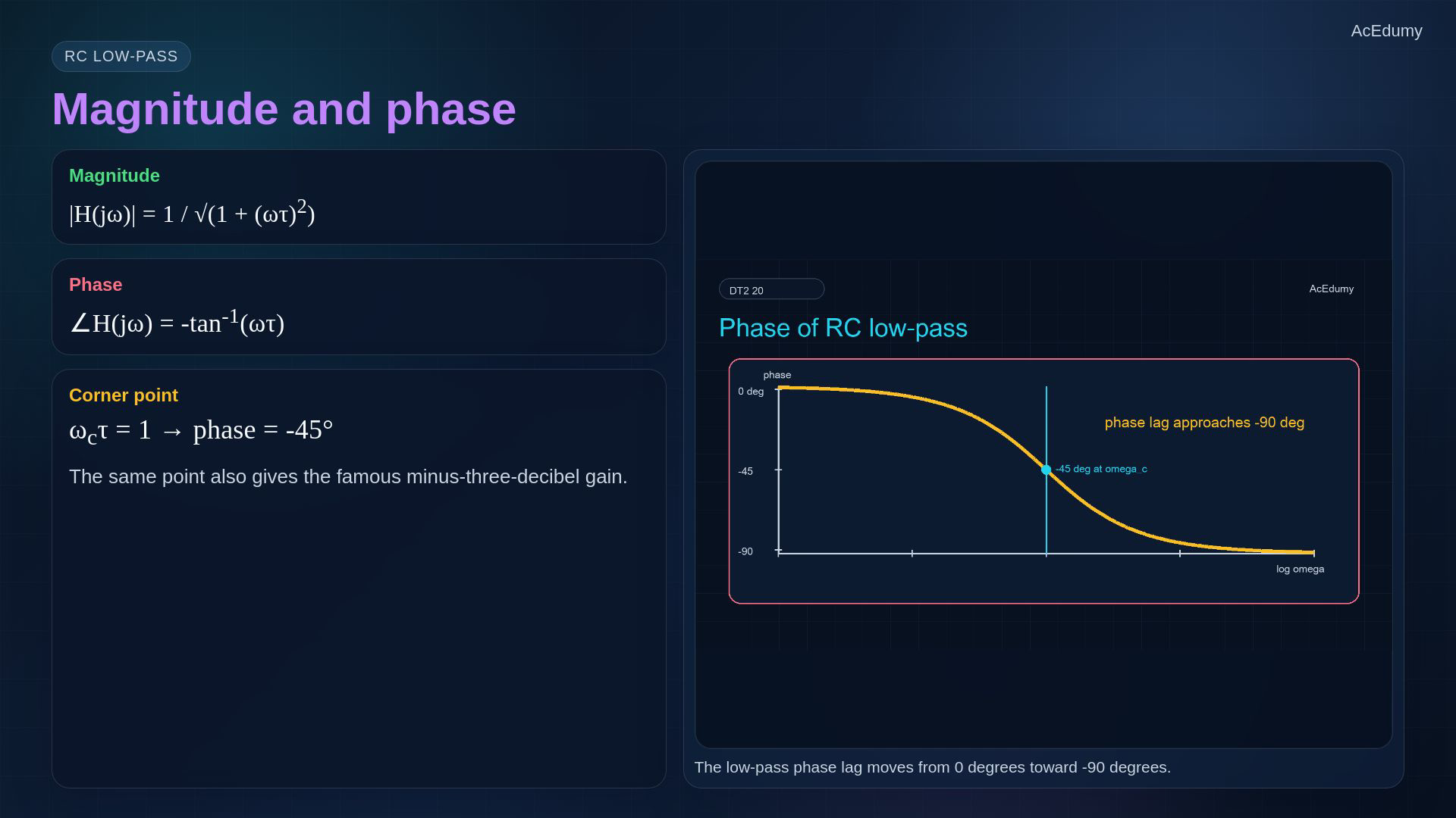
Reference from the existing video. The decibel-table and Bode-plot roles use readable traps and summary cards from the same final; full formulas and the required conditions are stated in the notebook. The entire dimensionless product is squared:For positive frequency the RC phase is negative:At very low positive frequency the gain tends to one and the phase tends to zero.At the corner, in degrees:At very high positive frequency the phase approaches minus ninety degrees.Narration transcript
From H of j omega equals one over one plus j omega tau, the magnitude is one over the square root of one plus omega tau squared. The phase is minus arctangent omega tau. At very low frequency, magnitude is almost one and phase is almost zero degrees. At the corner, omega tau equals one, the phase is minus forty-five degrees. At very high frequency, phase approaches minus ninety degrees.
6. Keep amplitude and power ratios distinct
Reference from the existing video. The decibel-table and Bode-plot roles use readable traps and summary cards from the same final; full formulas and the required conditions are stated in the notebook. A logarithmic scale makes a wide range of positive magnitude ratios readable.For a dimensionless voltage or current amplitude ratio r, the numerical gain in decibels is:Unity amplitude ratio gives zero decibels:This amplitude ratio gives approximately minus three decibels:One tenth and ten times amplitude give opposite gains in decibels:For a positive power ratio use:Narration transcript
Engineers usually plot amplitude ratios in decibels. For voltage or current amplitude ratios, d B equals twenty log base ten of the magnitude ratio. A ratio of one is zero d B. A ratio of one over square root of two is about minus three d B. A ratio of point one is minus twenty d B, and a ratio of ten is plus twenty d B. For power ratios, use ten log base ten instead.
7. Distinguish the exact RC curve from its asymptote
Reference from the existing video. The decibel-table and Bode-plot roles use readable traps and summary cards from the same final; full formulas and the required conditions are stated in the notebook. Use a logarithmic positive-frequency axis and amplitude gain measured in decibels.The angular corner frequency is the reciprocal time constant:At the corner the exact RC gain in decibels is:Well below the corner, the exact curve approaches zero decibels.Far above the corner, the slope approaches minus twenty decibels per decade; it is not exactly that slope just above the corner.Narration transcript
The Bode magnitude plot puts frequency on a log axis and gain in decibels. For the RC low-pass, the corner frequency is omega c equals one over tau. At that corner, the gain is minus three point zero one d B. Before the corner, the curve is close to zero d B. After the corner, it falls at about minus twenty d B per decade.
8. Keep units, impedance assumptions and phase signs
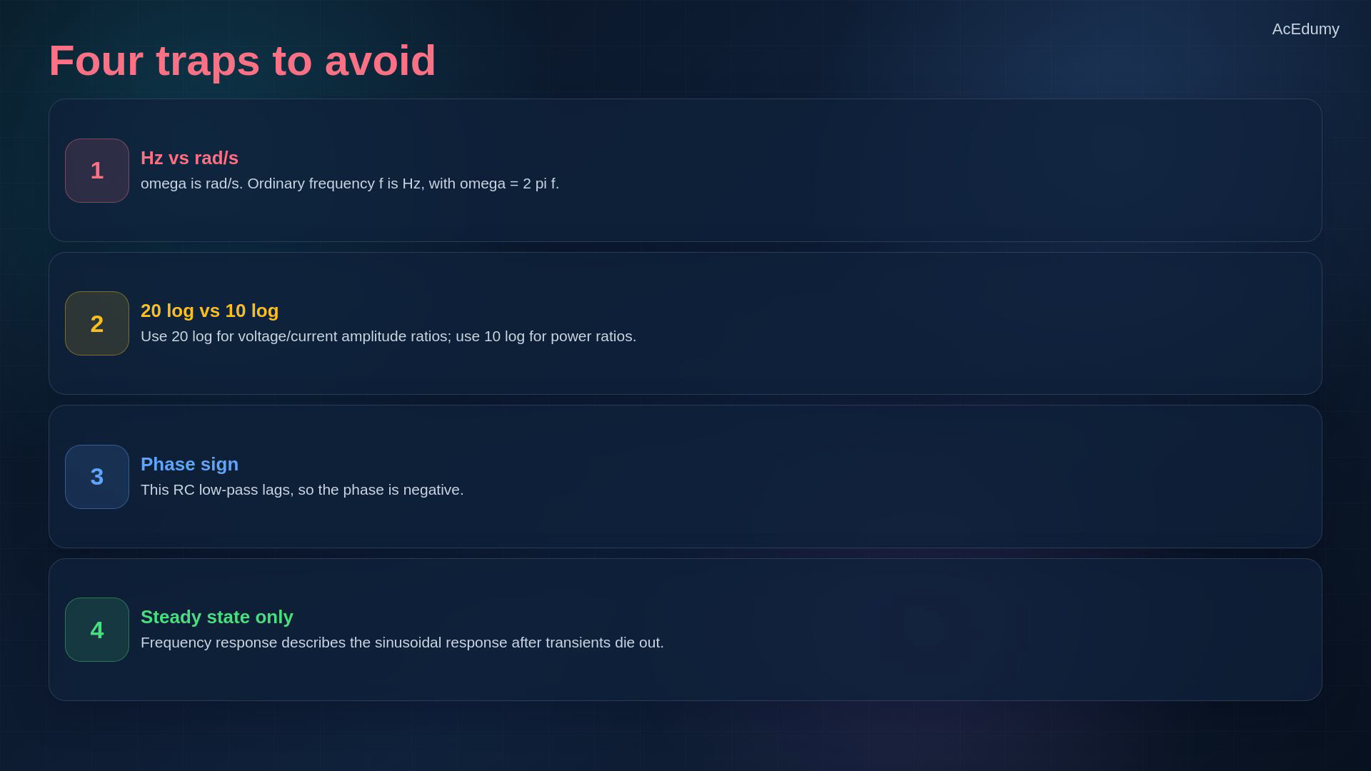
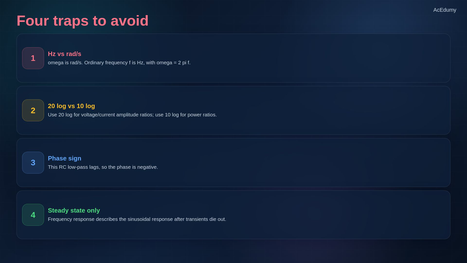
Reference from the existing video. The decibel-table and Bode-plot roles use readable traps and summary cards from the same final; full formulas and the required conditions are stated in the notebook. Four checks before reading a frequency-response plot.Angular frequency is in radians per second and ordinary frequency in hertz:Use twenty log for amplitude and ten log for power; equal-resistance conditions are needed to identify the amplitude result with the power gain.For positive frequency this RC voltage low-pass has a negative phase: it lags.This sinusoidal rule assumes decaying transients; an unstable or imaginary-axis-pole system need not settle.Narration transcript
Four common traps. First, omega is angular frequency in radians per second; ordinary frequency f is in hertz, and omega equals two pi f. Second, use twenty log for voltage or current amplitude ratios, but ten log for power ratios. Third, phase signs matter: this RC low-pass lags, so its phase is negative. Fourth, frequency response describes sinusoidal steady state after transients have died out.
9. Use the RC frequency-response landmarks
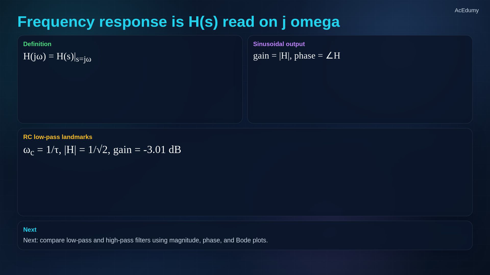
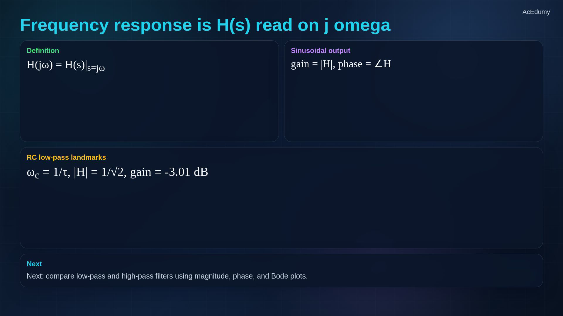
Reference from the existing video. The decibel-table and Bode-plot roles use readable traps and summary cards from the same final; full formulas and the required conditions are stated in the notebook. Summary: gain and phase are frequency-dependent properties.Start with the specified zero-state input-output transfer function.For a stable causal system, evaluate it on the imaginary axis:Keep amplitude gain, phase and logarithmic gain distinct; phase need not be a constant time delay.RC corner landmarks:Next: compare low-pass and high-pass magnitude, phase and Bode behavior.Narration transcript
Summary. Start from the transfer function H of s. Set s equal to j omega to get frequency response. The magnitude gives frequency-dependent gain, the angle gives phase shift, and decibels make wide ratio ranges easy to read. For the RC low-pass, the corner is one over tau, the gain is minus three d B there, and beyond it the magnitude falls at about minus twenty d B per decade. Next we can compare low-pass and high-pass filters using the same language.
Source video: Circuit Theory-2 #20 | Frequency Response and Decibels (4:50)