Antenna Theory — Problem Solving · Antenna Theory

#04 Friis transmission, free-space loss and received power

Solve the same ideal wireless link in watts and dBm, keeping gain references, propagation assumptions and rounding consistent.

Question

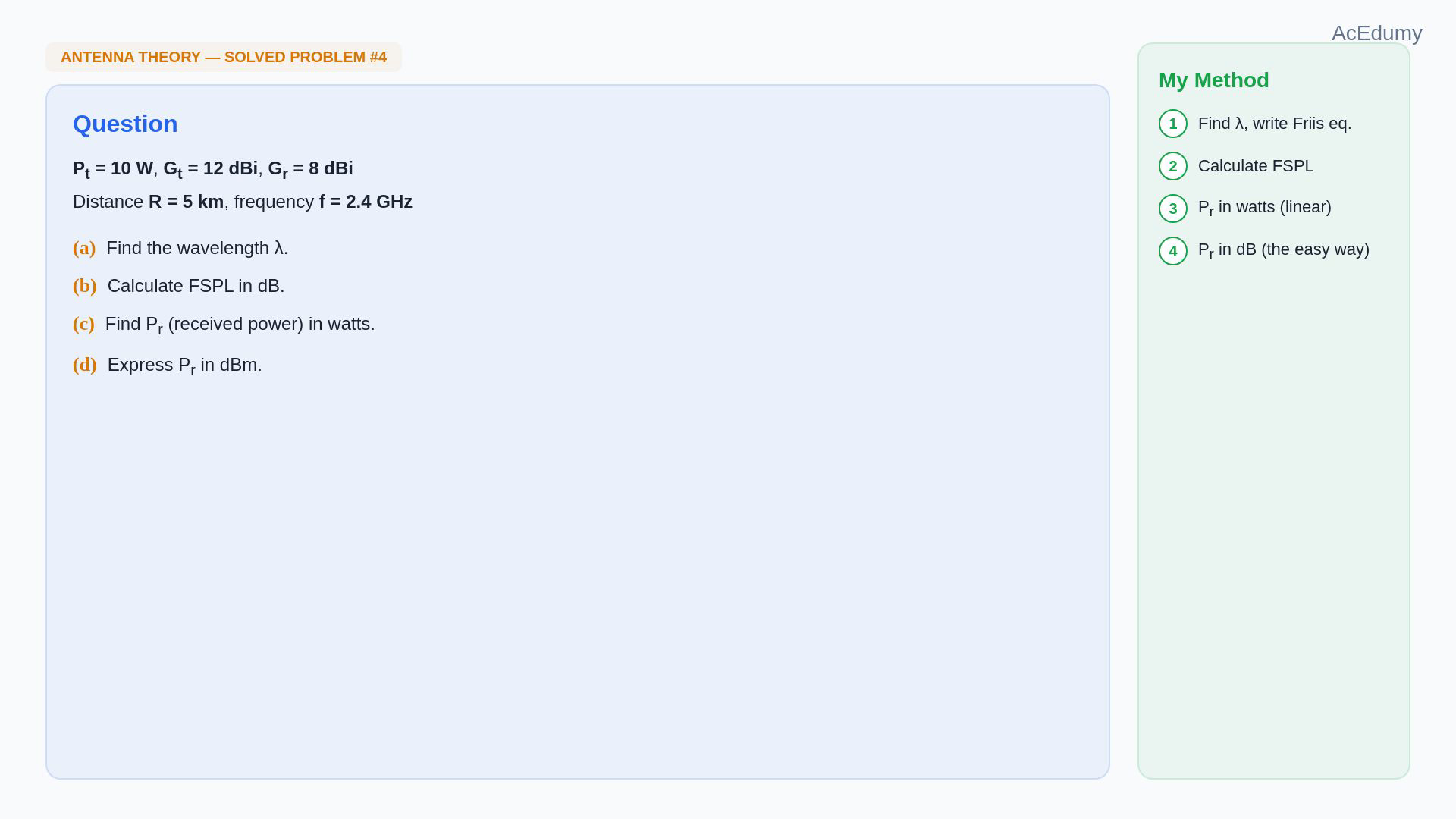
Original English link-budget reference showing the stated parameters, Friis propagation square, loss, linear received power, dBm budget or final results. — Use the stated free-space and matched-antenna assumptions. Numerical reference results are rounded; dBi gains become linear factors in Friis, and dBm powers use a one-milliwatt reference.

Calculate the received power for a 10 W transmitter, 12 dBi transmit gain, 8 dBi receive gain, 5 km separation and 2.4 GHz frequency. Find wavelength and free-space loss, then solve in watts and dBm and reconcile the rounding. Assume unobstructed free-space propagation in the far field of both antennas, gains evaluated along the line between them, matched polarization, matched receive loading and no additional feeder or propagation loss. Treat the transmit power as power accepted at the antenna input and the receive power as available to a matched load. Gain includes radiation efficiency; do not count it twice. The drawing is a qualitative link illustration, not a geometric or electromagnetic scale model. A ground plane in an illustration does not introduce a reflected ray into the free-space calculation. Use the stated approximation c of 3 times ten to the eighth metres per second. Lambda is c divided by f, giving 0.125 m or 12.5 cm. The normalized power propagation factor is the square of the entire dimensionless ratio lambda/(4 pi R). The narration's “all squared” applies to that last ratio only, as its following explanation and actual equation card show; transmit power and antenna gains are not squared. Consistent distance and wavelength units are essential. Let L denote the positive dimensionless free-space loss. L=(4 pi R/lambda)^2, while received power is P_t G_t G_r/L. The unsquared ratio is about 502654.8246 and L about 2.5266187 times ten to the eleventh. The source values 502655 and 2.527 times ten to the eleventh are rounded. “Power lost” here describes the small fraction coupled into the receiver, not absorption or destruction of the entire transmitted power. Flux density at the receive location is P_t G_t/(4 pi R^2), and the matched effective aperture is G_r lambda^2/(4 pi); their product independently gives Friis. The linear gains are ten raised to 12/10 and 8/10, about 15.84893 and 6.30957. Their unrounded product is exactly 100 for the stated dBi numbers. Thus the numerator is 1000 W. Using the displayed rounded gains gives 1000.135 W, displayed as about 1000 or 1000.1 W. The precise ideal result is about 3.9578587 nanowatts, correctly rounded to 3.96 nanowatts. Equalities next to rounded source numbers should be read at their displayed precision. For the logarithmic equation, define lowercase p_t and p_r as numerical power levels in dBm, lowercase g_t and g_r as numerical gains in dBi, and L_d as the numerical loss in dB. Each dBm value is ten times the base-ten logarithm of power divided by one milliwatt; dBi uses dimensionless gain relative to an isotropic antenna. L_d is ten times the base-ten logarithm of L, equivalently twenty times the logarithm of the unsquared distance ratio. Arguments of logarithms are dimensionless and positive. These are power quantities, so applying twenty times the logarithm directly to L or to watts would be wrong. Ten watts corresponds to 40 dBm or 10 dBW. The unrounded loss is about 114.0253971 dB, giving about −54.0253971 dBm. With the source's rounded 114 dB, the arithmetic 40+12+8−114 gives −54 dBm exactly for those rounded inputs. Converting this rounded level back gives about 3.9810717 nanowatts, rounded to 3.98 nanowatts. Both routes agree at their intended precision; 3.96 and 3.98 are not asserted to be identical exact numbers. A negative dBm level represents positive power below one milliwatt, not negative physical power. The power in watts is one thousandth of ten raised to p_r/10. At fixed frequency and gains, doubling distance quarters received power and increases free-space loss by about 6.0206 dB. At fixed distance and gains, doubling frequency has the same factor. A claim at fixed physical antenna aperture requires accounting for frequency-dependent gain instead. Additional loss factors at least one divide the linear received power and subtract their positive dB values. Antenna gain redistributes radiation and receiving coupling; it does not generate extra energy. The approximate four-nanowatt signal may suit a receiver, but this requires its noise, bandwidth, interference and detection requirements; the power estimate alone does not guarantee a working real link. Friis supplies the ideal propagation term, while a complete practical budget needs the actual environment and margins. The original reference equations are readable. In the path-loss frame a divider and nearby heading crowd the intermediate loss value, but the number, exponent and completed final loss remain visible. Read the FSPL label as the dimensionless loss in its linear equation and as its explicitly labelled dB value in the result box. The source's shorthand dB power label means the specified dBm reference. The final Friis and dB equations preserve the propagation square and the negative received level.

Written solution and narration transcript(shows the full solution)

Below are all the lines written in the notebook together with the full narration transcript.

1. Read the link parameters
Use the stated free-space and matched-antenna assumptions. Numerical reference results are rounded; dBi gains become linear factors in Friis, and dBm powers use a one-milliwatt reference.
Set up the fourth solved problem: an ideal free-space link budget.
The transmit power is 10 W and the transmit antenna gain is 12 dBi.
The receive antenna is 5 km away and has 8 dBi gain.
The frequency is 2.4 GHz.
Find wavelength, free-space loss, received watts and received dBm.
Proceed through wavelength, path loss, linear power and the dB budget.
Narration transcript
Here's our fourth problem, and this time it's a real-world link budget calculation. A transmitter sends ten watts through an antenna with twelve dBi gain. Five kilometers away, a receive antenna with eight dBi gain picks up the signal. The frequency is two-point-four gigahertz — the Wi-Fi band. We need to find the wavelength, the path loss, and the received power — both in watts and in dBm. Let's follow our four-step method.
2. Set the wavelength and Friis model
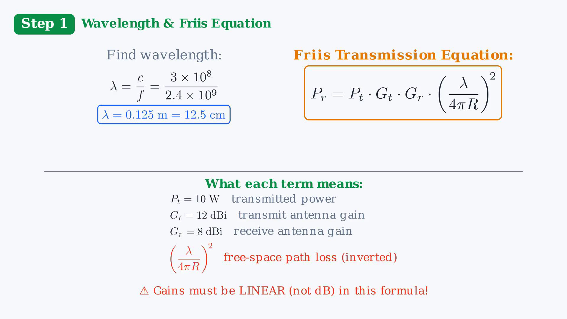
Use the stated free-space and matched-antenna assumptions. Numerical reference results are rounded; dBi gains become linear factors in Friis, and dBm powers use a one-milliwatt reference.
Find the wavelength and specify the Friis model.
$\displaystyle \lambda =\frac{ c}{f}$
Using the stated speed approximation gives 0.125 m, or 12.5 cm.
Write Friis with the square applied to the last propagation factor.
$\displaystyle P_{r} = P_{t} G_{t} G_{r} \left(\frac{\lambda }{4 \pi R}\right)^{2}$
Define the power, gain and distance references consistently.
The transmitted power accepted by the antenna is 10 W in this model.
Use the antenna gains in the directions of the other antenna.
The squared wavelength-to-distance factor is the inverse of free-space loss; spreading reduces captured power without dissipating all transmitted energy.
Use dimensionless linear gains in the multiplicative equation.
Convert the given dBi gains before substitution.
Narration transcript
Step one: find the wavelength and set up the Friis equation. Lambda equals c over f: three times ten to the eighth divided by two-point-four times ten to the ninth. That gives us zero-point-one-two-five meters, or twelve-point-five centimeters. Now the Friis transmission equation. P-r equals P-t times G-t times G-r times lambda over four-pi-R, all squared. Let me explain each term. P-t is the transmitted power: ten watts. G-t and G-r are the antenna gains. And that last factor, lambda over four-pi-R squared, is the inverse of the free-space path loss — it tells you how much power is lost just from the signal spreading out over distance. One critical note: the gains in this formula must be linear, not in dB. We'll handle that conversion.
3. Calculate free-space path loss
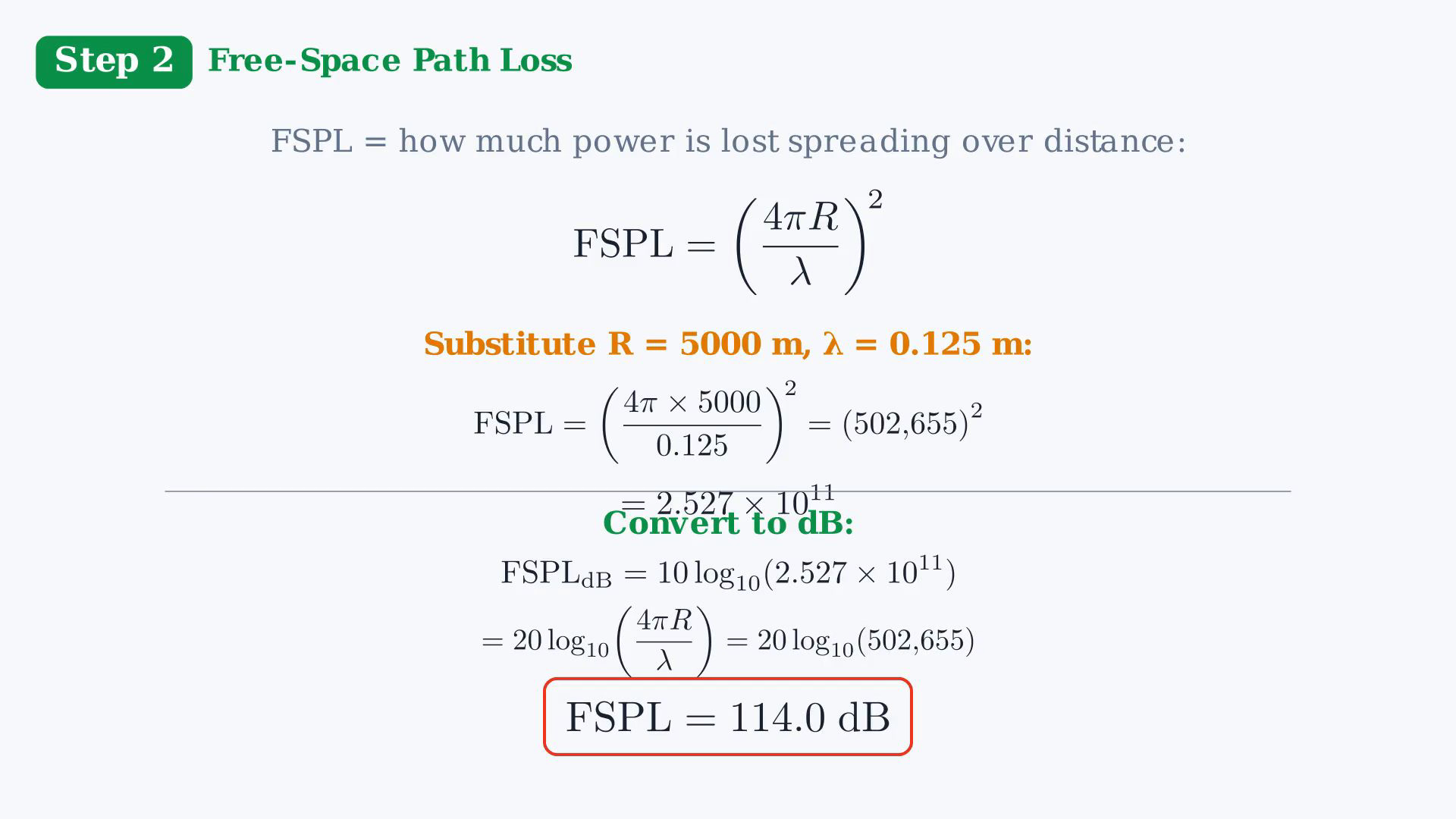
Use the stated free-space and matched-antenna assumptions. Numerical reference results are rounded; dBi gains become linear factors in Friis, and dBm powers use a one-milliwatt reference.
Calculate the dimensionless free-space loss L.
$\displaystyle L = \left(\frac{4 \pi R}{\lambda }\right)^{2}$
Use 5000 m and 0.125 m; the unsquared ratio is about 502655.
Its square is about 2.527 times ten to the eleventh.
This large loss ratio describes weak coupling to the receiving antenna.
Twenty times the base-ten logarithm of the unsquared ratio is about 114 dB.
Retain additional digits internally when comparing linear and dB calculations.
Narration transcript
Step two: calculate the free-space path loss. FSPL equals four-pi-R over lambda, all squared. Substituting R equals five thousand meters and lambda equals zero-point-one-two-five meters: four-pi times five thousand divided by zero-point-one-two-five gives five-hundred-two-thousand-six-fifty-five. Square that and we get two-point-five-two-seven times ten to the eleventh. That's a huge number — signals lose a LOT of power over five kilometers. In dB: twenty log-ten of five-oh-two-six-five-five equals one-hundred-fourteen dB. That's our path loss.
4. Calculate received power in watts
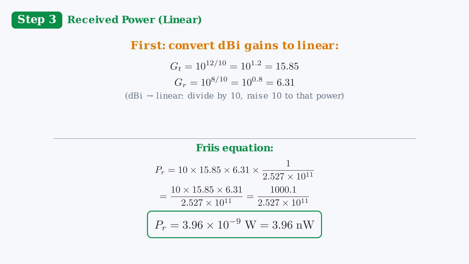
Use the stated free-space and matched-antenna assumptions. Numerical reference results are rounded; dBi gains become linear factors in Friis, and dBm powers use a one-milliwatt reference.
Calculate received power in watts.
Convert each gain from dBi to a dimensionless power gain.
$\displaystyle G_{t} = 10^{12/10} = 10^{1.2}$
$\displaystyle G_{r} = 10^{8/10} = 10^{0.8}$
$\displaystyle P_{r} =\frac{ P_{t} G_{t} G_{r}}{L}$
The rounded gains 15.85 and 6.31 give a numerator of about 1000 W.
The loss denominator is about 2.5 times ten to the eleventh.
The received power is about 3.96 nanowatts, or roughly 4 nanowatts.
Receiver usability also depends on bandwidth, noise, interference and the required signal quality.
Narration transcript
Step three: calculate received power the direct way, in watts. First we need to convert the gains from dBi to linear. G-t equals ten to the power of twelve over ten, which is ten to the one-point-two, which is fifteen-point-eight-five. G-r equals ten to the power of eight over ten, which is ten to the zero-point-eight, which is six-point-three-one. Now plug everything into Friis: ten watts times fifteen-point-eight-five times six-point-three-one, divided by two-point-five-two-seven times ten to the eleventh. The numerator is about one thousand. The denominator is two-point-five times ten to the eleventh. Result: three-point-nine-six times ten to the minus nine watts, or about four nanowatts. That's tiny — but a good receiver can work with that.
5. Convert to a dB budget
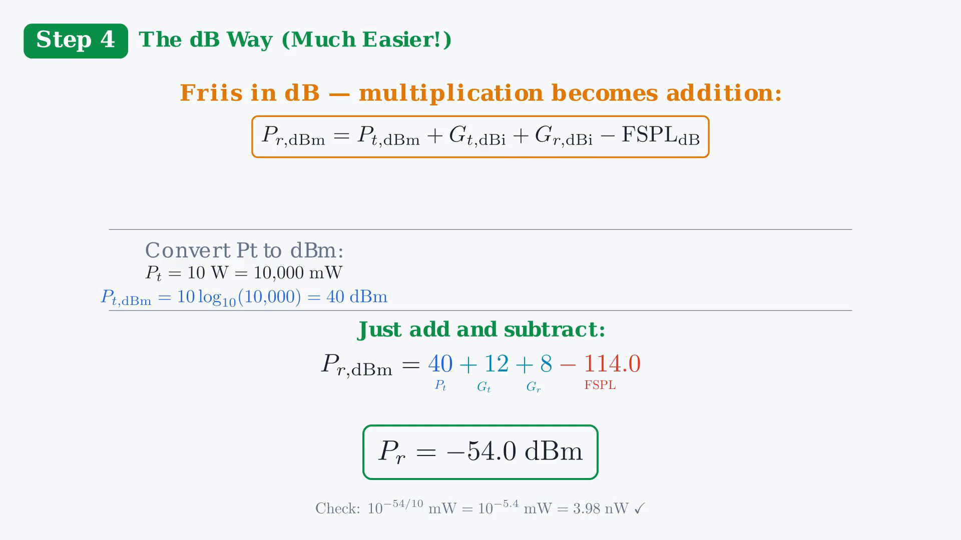
Use the stated free-space and matched-antenna assumptions. Numerical reference results are rounded; dBi gains become linear factors in Friis, and dBm powers use a one-milliwatt reference.
Express the same power budget using logarithmic values.
$\displaystyle p_{r} = p_{t} + g_{t} + g_{r} - L_{d}$
Ten watts is 10000 milliwatts, corresponding to 40 dBm.
$\displaystyle p_{r} = 40 + 12 + 8 - 114$
$\displaystyle p_{r} = -54$
Converting the rounded −54 dBm back gives about 3.98 nanowatts.
The small difference from 3.96 nanowatts comes from rounding the path loss.
Logarithms turn products and quotients of positive ratios into sums and differences.
Narration transcript
Step four: the same calculation in dB — and this is MUCH easier. In dB, the Friis equation becomes just addition and subtraction: P-r in dBm equals P-t in dBm plus G-t in dBi plus G-r in dBi minus FSPL in dB. First convert P-t to dBm: ten watts is ten thousand milliwatts, so ten-log-ten of ten thousand equals forty dBm. Now just add: forty plus twelve plus eight minus one-fourteen. That's sixty minus one-fourteen, which equals minus fifty-four dBm. Quick check: ten to the minus five-point-four milliwatts equals three-point-nine-eight nanowatts. Matches our linear answer. This is why engineers work in dB — multiplication becomes addition, and you can do the entire link budget in your head.
6. Interpret the free-space link
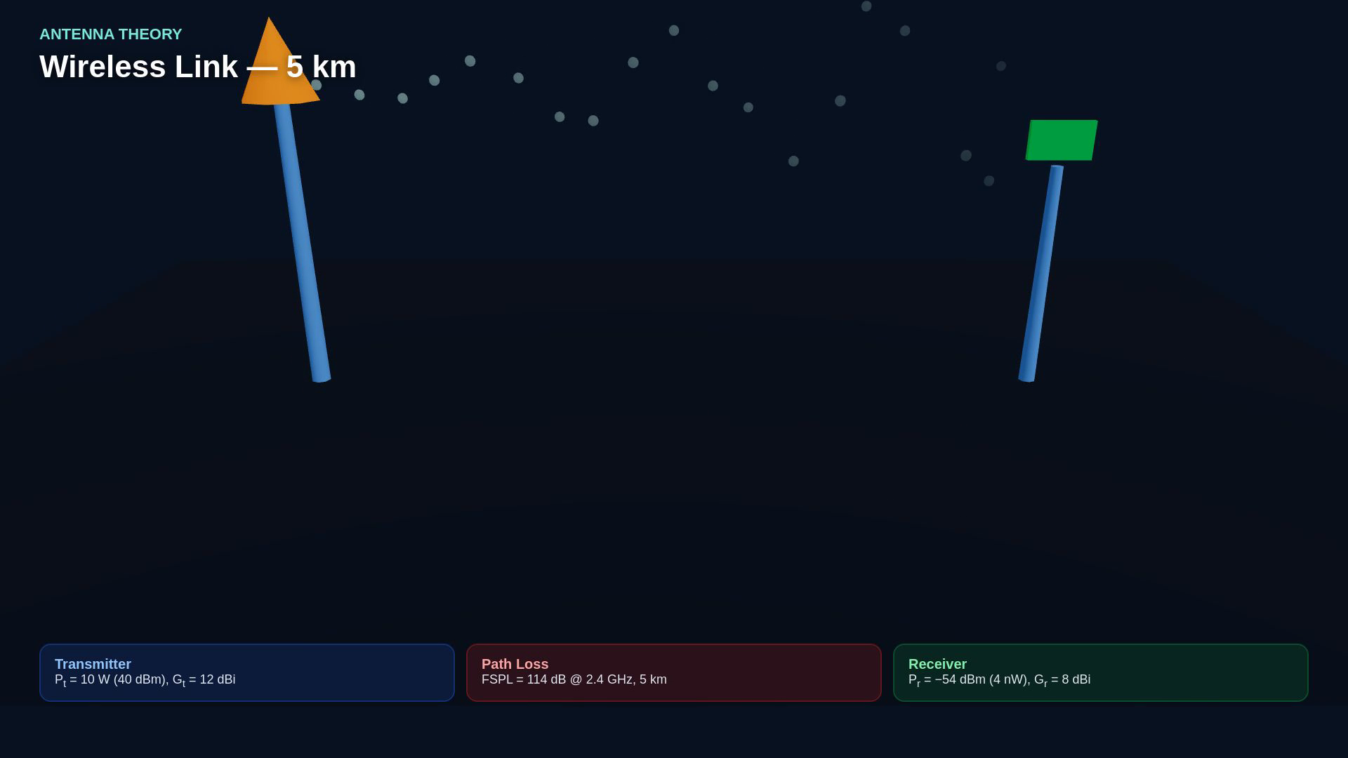
Use the stated free-space and matched-antenna assumptions. Numerical reference results are rounded; dBi gains become linear factors in Friis, and dBm powers use a one-milliwatt reference.
Interpret the link model.
The drawing represents transmitter and receiver separated by 5 km.
Power spreads geometrically; free-space loss is not absorption of all radiated power.
Directional antenna gain and receive aperture improve coupling without creating energy.
For the stated ideal parameters, 10 W transmitted gives about 4 nW received, approximately −54 dBm.
Real link budgets add actual propagation, feeder, mismatch and operating-margin terms.
Narration transcript
Here's the big picture. Transmitter on the left, receiver on the right, five kilometers apart. The signal spreads out as it travels — that's the path loss. But the antenna gains focus the energy, partially compensating for the loss. The net result: ten watts in, four nanowatts out, minus fifty-four dBm. This is the foundation of every wireless link design.
7. Collect and check the results
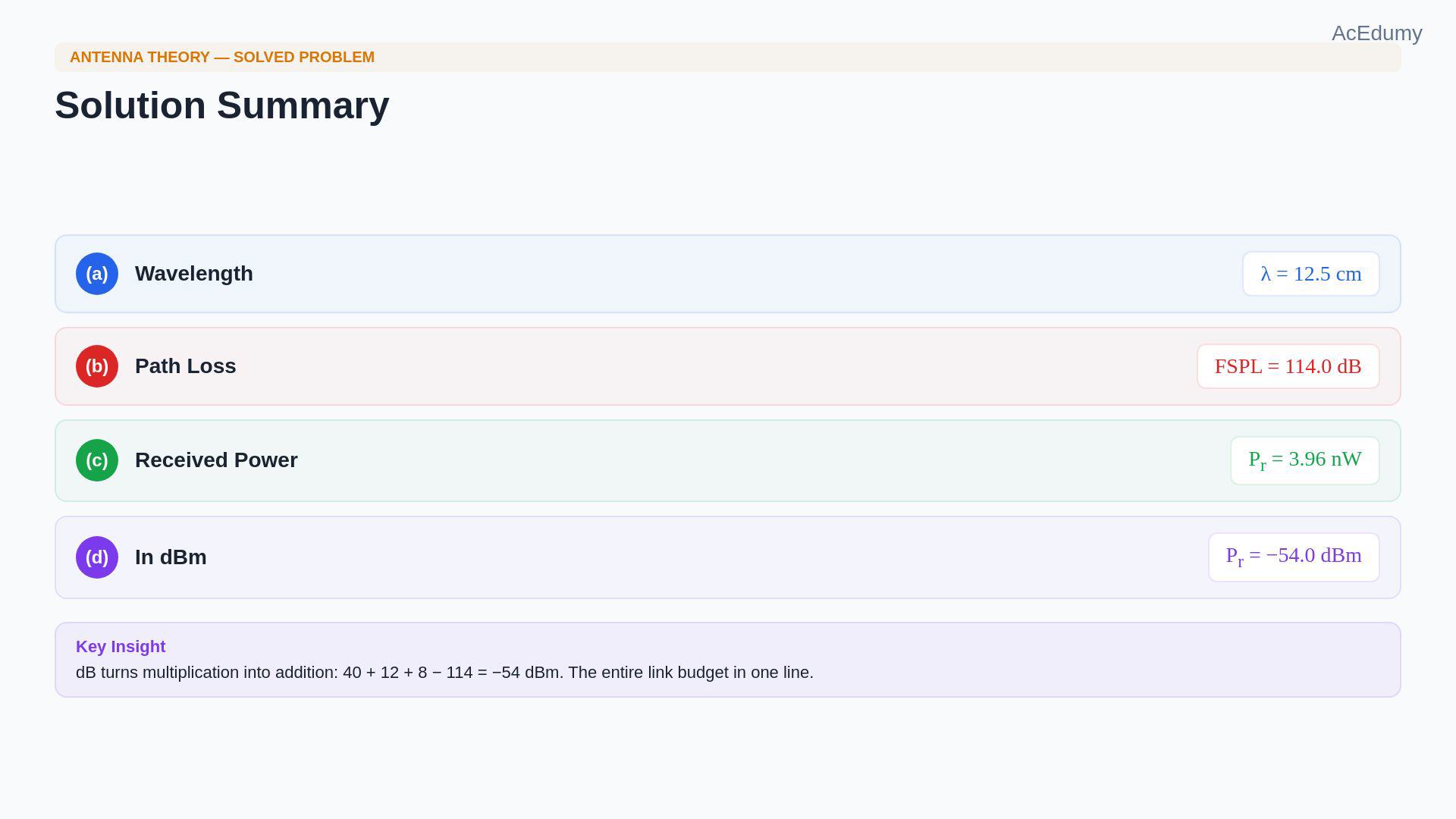
Use the stated free-space and matched-antenna assumptions. Numerical reference results are rounded; dBi gains become linear factors in Friis, and dBm powers use a one-milliwatt reference.
Collect the four results with their units and precision.
The wavelength is 12.5 cm using the stated speed approximation.
Free-space loss is about 114 dB.
The received power is about 3.96 nanowatts.
The same received power is about −54 dBm.
Multiplication and division in the linear budget become addition and subtraction in the dB budget.
$\displaystyle 40 + 12 + 8 - 114 = -54$
Keep dBm power levels, dBi antenna gains and dB loss values distinct.
Narration transcript
Let's box our answers. Part a: lambda equals twelve-point-five centimeters. Part b: free-space path loss equals one-hundred-fourteen dB. Part c: received power equals three-point-nine-six nanowatts. Part d: minus fifty-four dBm. The key insight: working in dB turns a messy multiplication into simple addition. Forty plus twelve plus eight minus one-fourteen. That's the entire link budget in one line.