#28 Integration conventions, impulse pairs and rectangular-pulse transform

Below are all the lines written in the notebook together with the full narration transcript.

1. 1. Transform and inversion conventions

   

   For the ordinary forward transform, use a finite Lebesgue integral of a measurable signal:

   $\displaystyle X\left(\omega \right)=\int _{-\infty }^{\infty }x\left(t\right)e^{-j\omega t}\mathrm{d}t$

   When the applicable inversion conditions hold, the inverse uses the opposite exponent sign and normalization:

   $\displaystyle x\left(t\right)=\left(\frac{1}{2\pi }\right)\int _{-\infty }^{\infty }X\left(\omega \right)e^{j\omega t}d \omega$

   Absolute integrability guarantees the forward integral; it does not by itself guarantee an absolutely integrable inverse spectrum.

   Conditional improper integrals and generalized transforms use different existence conventions and must be identified explicitly.

   We will distinguish those conventions while evaluating shifted impulses, impulse pairs and a finite rectangular pulse.

   Narration transcript

   In the previous video, we derived the Fourier Transform and its inverse by letting the period of a periodic extension go to infinity. Now we have two powerful formulas: X of omega equals the integral of x of t times e to the minus j omega t, and x of t equals one over two pi times the integral of X of omega times e to the plus j omega t. But does this integral always converge? And what does the Fourier Transform look like for specific signals? In this video, we'll first establish the convergence condition, then compute our first Fourier Transform examples: impulse functions, impulse pairs, and the rectangular pulse.

2. 2. Absolute-integral bound

   

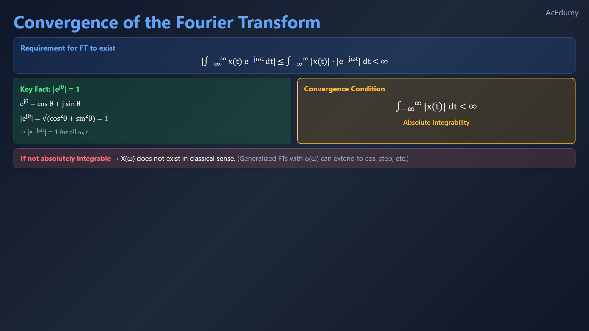
   For a measurable signal, define its absolute-integral size; the finite Lebesgue convention requires this quantity to be finite:

   $\displaystyle I_{1}=\int _{-\infty }^{\infty }|x\left(t\right)|dt$

   The triangle inequality supplies a sufficient bound:

   $\displaystyle |X\left(\omega \right)|\le B\left(\omega \right)=\int _{-\infty }^{\infty }|x\left(t\right)||e^{-j\omega t}|dt$

   The unit-magnitude fact applies to a purely imaginary exponent with real angle, real time and real angular frequency.

   Euler identity for a real angle is:

   $\displaystyle e^{j\theta }=\cos \left(\theta \right)+j \sin \left(\theta \right)$

   The squared trigonometric components give unit magnitude:

   $\displaystyle |e^{j\theta }|=\sqrt{\cos \left(\theta \right)^{2}+\sin \left(\theta \right)^{2}}=1$

   The oscillatory factor leaves the absolute-integral size unchanged:

   $\displaystyle |e^{-j\omega t}|=1, B\left(\omega \right)=I_{1}$

   A finite absolute-integral size means absolute integrability, or membership in L1.

   Every L1 signal has a finite forward transform at every real frequency. Necessity here follows from the finite Lebesgue definition, not by reversing the triangle inequality.

   Outside L1, a finite Lebesgue transform is unavailable, but a conditionally convergent ordinary improper transform may still exist.

   Generalized transforms provide another extension for impulses, cosines and steps; they do not turn a Dirac impulse into an ordinary L1 function.

   Narration transcript

   For the Fourier Transform integral to have a finite value, we need: the absolute value of the integral from negative infinity to infinity of x of t, e to the minus j omega t, dt must be less than infinity. Using the triangle inequality, this is less than or equal to the integral of the absolute value of x of t, times the absolute value of e to the minus j omega t, dt. Now here's a key fact. The magnitude of a complex exponential is always one. Since e to the j theta equals cosine theta plus j sine theta, its magnitude is the square root of cosine squared theta plus sine squared theta, which equals one. Therefore, the absolute value of e to the minus j omega t equals one, and our condition simplifies to: the integral from negative infinity to infinity of the absolute value of x of t, dt must be finite. This is called absolute integrability. If a signal is absolutely integrable, its Fourier Transform exists. If not, the transform may not converge in the ordinary sense. Note however that generalized Fourier Transforms using delta functions can extend this to signals like cosines and step functions.

3. 3. Impulse examples

   

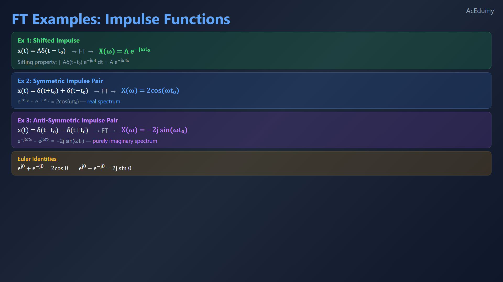
   Interpret impulses as point measures or distributions; use real shift and amplitude parameters, with positive shift size for the distinct pairs.

   The first signal is a shifted impulse with weight A:

   $\displaystyle x\left(t\right)=A\delta \left(t-t_{0}\right)$

   The sifting property evaluates the Fourier kernel at the impulse location:

   $\displaystyle X\left(\omega \right)=\int _{-\infty }^{\infty }A\delta \left(t-t_{0}\right)e^{-j\omega t}\mathrm{d}t=A e^{-j\omega t_0}$

   Its phase varies with frequency while its magnitude equals the impulse weight magnitude:

   $\displaystyle |X\left(\omega \right)|=|A|$

   Define the symmetric pair with two positive unit weights:

   $\displaystyle x_{S}\left(t\right)=\delta \left(t+t_{0}\right)+\delta \left(t-t_{0}\right)$

   The symmetric pair is real and even; the impulse at negative time contributes the positive-exponent kernel.

   Linearity gives the sum of the two kernel values:

   $\displaystyle X_{S}\left(\omega \right)=e^{j\omega t_0}+e^{-j\omega t_0}$

   Euler identity reduces that sum to a real even spectrum:

   $\displaystyle X_{S}\left(\omega \right)=2\cos \left(\omega t_{0}\right)$

   The antisymmetric pair has positive weight at positive time and negative weight at negative time:

   $\displaystyle x_{A}\left(t\right)=\delta \left(t-t_{0}\right)-\delta \left(t+t_{0}\right)$

   This pair is real and odd; preserving which impulse is subtracted determines the transform sign.

   Its transform is purely imaginary and odd:

   $\displaystyle X_{A}\left(\omega \right)=e^{-j\omega t_0}-e^{j\omega t_0}=-2j \sin \left(\omega t_{0}\right)$

   The symmetric pair gives a cosine spectrum; reversing the antisymmetric weights would reverse the imaginary sine spectrum.

   Narration transcript

   Let's compute our first examples. Example one: find the Fourier Transform of a single impulse: x of t equals A times delta of t minus t-zero. Applying the FT integral and using the sifting property of the delta function: X of omega equals the integral of A delta of t minus t-zero, times e to the minus j omega t, dt, which equals A times e to the minus j omega t-zero. So a shifted impulse maps to a complex exponential in the frequency domain. Example two: find X of omega for x of t equals delta of t plus t-zero, plus delta of t minus t-zero. This is a symmetric pair of impulses. Using linearity: X of omega equals e to the plus j omega t-zero, plus e to the minus j omega t-zero. By Euler's formula, this equals two cosine of omega t-zero. Example three: x of t equals delta of t minus t-zero, minus delta of t plus t-zero. This is an anti-symmetric pair. The transform gives: X of omega equals e to the minus j omega t-zero, minus e to the plus j omega t-zero, which equals minus two j sine of omega t-zero. Notice: symmetric impulse pairs give a real cosine spectrum, while anti-symmetric pairs give a purely imaginary sine spectrum.

4. 4. Rectangular pulse and normalized sinc

   

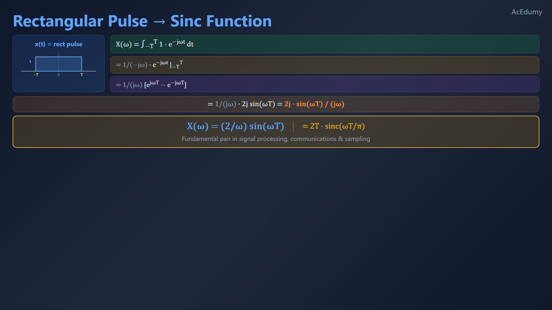
   Let the half-width T be positive and use real angular frequency. The pulse has total width twice T.

   The rectangular pulse is one between negative T and positive T and zero outside; endpoint values do not affect its forward integral.

   Only the finite support contributes:

   $\displaystyle X\left(\omega \right)=\int _{-T}^{T}e^{-j\omega t}\mathrm{d}t$

   For nonzero angular frequency, an antiderivative of the kernel is:

   $\displaystyle g\left(t\right)=\frac{e^{-j\omega t}}{-j\omega }$

   Evaluate the upper endpoint minus the lower endpoint:

   $\displaystyle X\left(\omega \right)=\frac{e^{-j\omega T}-e^{j\omega T}}{-j\omega }$

   Reverse both signs to obtain the equivalent expression:

   $\displaystyle X\left(\omega \right)=\frac{e^{j\omega T}-e^{-j\omega T}}{j\omega }$

   Euler identity supplies the numerator:

   $\displaystyle e^{j\omega T}-e^{-j\omega T}=2j \sin \left(\omega T\right)$

   Cancel the imaginary unit for nonzero angular frequency:

   $\displaystyle X\left(\omega \right)=\frac{2\sin \left(\omega T\right)}{\omega }$

   Define normalized sinc as q, extending it continuously by q at zero equal to one:

   $\displaystyle q\left(z\right)=\frac{\sin \left(\pi z\right)}{\pi z}, X\left(\omega \right)=2T q\left(\frac{\omega T}{\pi }\right)$

   At zero frequency, direct integration gives the pulse area and removes the apparent singularity:

   $\displaystyle X\left(0\right)=2T$

   Narration transcript

   Now let's compute one of the most important Fourier Transform pairs in signal processing. Let x of t be a rectangular pulse of amplitude one, extending from minus capital T to plus capital T. Applying the FT definition: X of omega equals the integral from minus T to T of one times e to the minus j omega t, dt. Integrating the exponential: this equals e to the minus j omega t, divided by minus j omega, evaluated from minus T to T. Substituting the limits: one over minus j omega, times the quantity e to the minus j omega T, minus e to the plus j omega T. Rearranging: one over j omega, times the quantity e to the j omega T, minus e to the minus j omega T. The numerator is exactly two j sine of omega T by Euler's formula. So X of omega equals two j sine of omega T, divided by j omega, which simplifies to two sine of omega T, divided by omega. This can also be written as two T times sinc of omega T over pi, where sinc of x equals sine of pi x over pi x. This rectangular pulse to sinc function relationship is fundamental and appears throughout signal processing, communications, and sampling theory.

5. 5. Summary

   

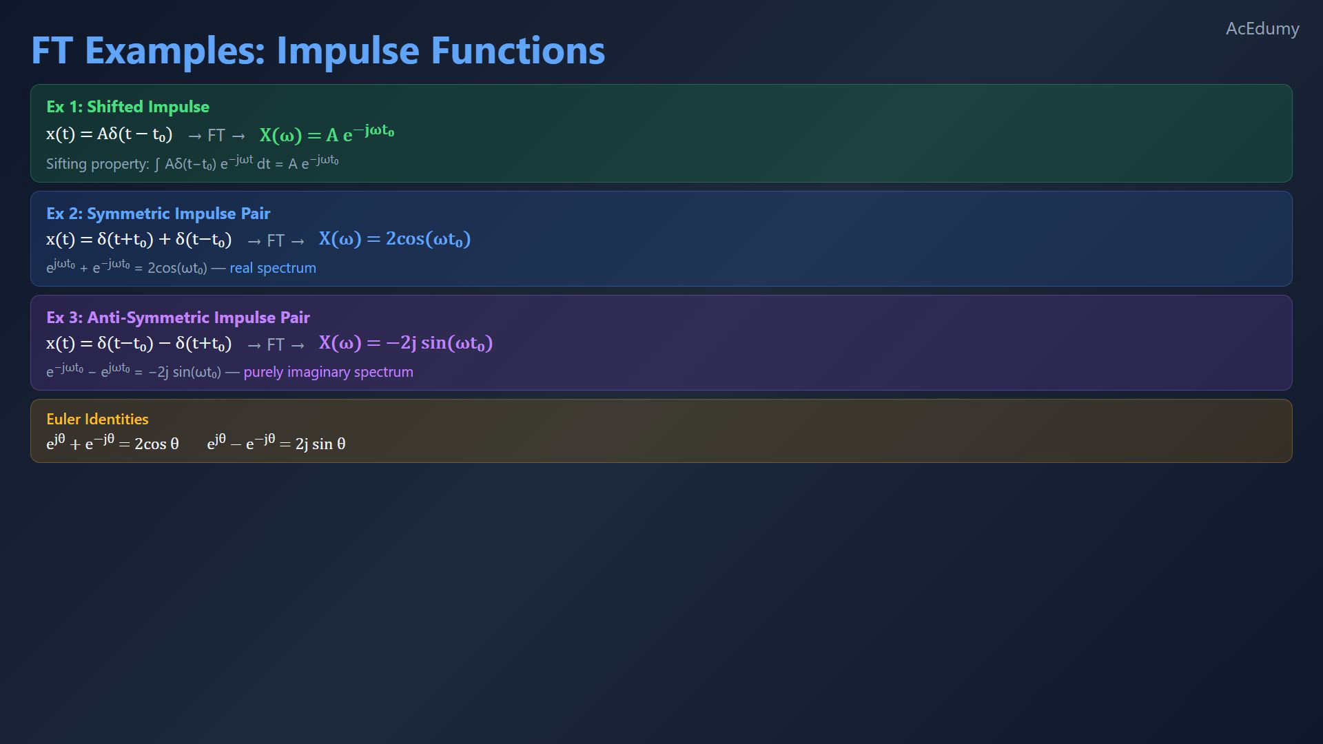
   Keep finite Lebesgue integration, conditional improper convergence and generalized transforms distinct.

   Under the stated finite Lebesgue convention, an ordinary signal must be absolutely integrable; this necessity does not apply to every other transform convention.

   The impulse examples use the generalized or point-measure interpretation, while the rectangular pulse is an ordinary L1 signal.

   The shifted impulse gives:

   $\displaystyle X\left(\omega \right)=A e^{-j\omega t_0}$

   The symmetric unit-impulse pair gives:

   $\displaystyle X_{S}\left(\omega \right)=2\cos \left(\omega t_{0}\right)$

   The rectangular pulse gives the normalized-sinc expression at every real frequency:

   $\displaystyle X\left(\omega \right)=2T q\left(\frac{\omega T}{\pi }\right)$

   Check exponent signs, impulse weights, pulse width and the zero-frequency limit before using a transform pair.

   The next topic relates Fourier series to the Fourier transform and develops further transform pairs.

   Narration transcript

   Let's summarize what we've learned. First, the convergence condition: a signal must be absolutely integrable for its Fourier Transform to exist in the classical sense. Second, we computed three key FT pairs. A shifted impulse A delta of t minus t-zero transforms to A e to the minus j omega t-zero. A symmetric impulse pair transforms to two cosine of omega t-zero. And a rectangular pulse from minus T to T transforms to two over omega times sine of omega T. These are building blocks that we'll use extensively. In the next video, we'll explore the relationship between Fourier Series and the Fourier Transform, and build a comprehensive table of transform pairs.

Source video: Signals & Systems #28 | FT Convergence & Basic Transform Examples (6:24)