Antenna Theory · Half-wave dipole normalized pattern, HPBW, and directivity
#13 Problem Solving 01 | Half-Wave Dipole Pattern and Directivity
Build the half-wave dipole's normalized field pattern, then calculate its half-power angles, HPBW, and directivity in linear units and dBi.
Question

A thin half-wave dipole of total length L=λ/2 is placed along the z axis in free space with current I(z)=I₀cos(kz). Write the normalized far-field pattern Eₙ(θ); identify its maximum and null directions; solve the half-power angles and HPBW; then calculate directivity in linear units and dBi from the radiation integral. Check the field-versus-power distinction, axial limits, and numerical rounding.
Written solution and narration transcript(shows the full solution)
Below are all the lines written in the notebook together with the full narration transcript.
1. Separate the problem into pattern, HPBW, and directivity outputs
The same normalized field pattern determines the axial nulls, the 78-degree HPBW, and the 2.15 dBi directivity. Here's our problem.A half-wave dipole antenna is oriented along the z-axis in free space.We need to find three things: the normalized radiation pattern, the half-power beamwidth, and the directivity in dBi.Let's follow our method card step by step.Narration transcript
Here's our problem. A half-wave dipole antenna is oriented along the z-axis in free space. We need to find three things: the normalized radiation pattern, the half-power beamwidth, and the directivity in dBi. Let's follow our method card step by step.
2. Set up the half-wave dipole geometry and current
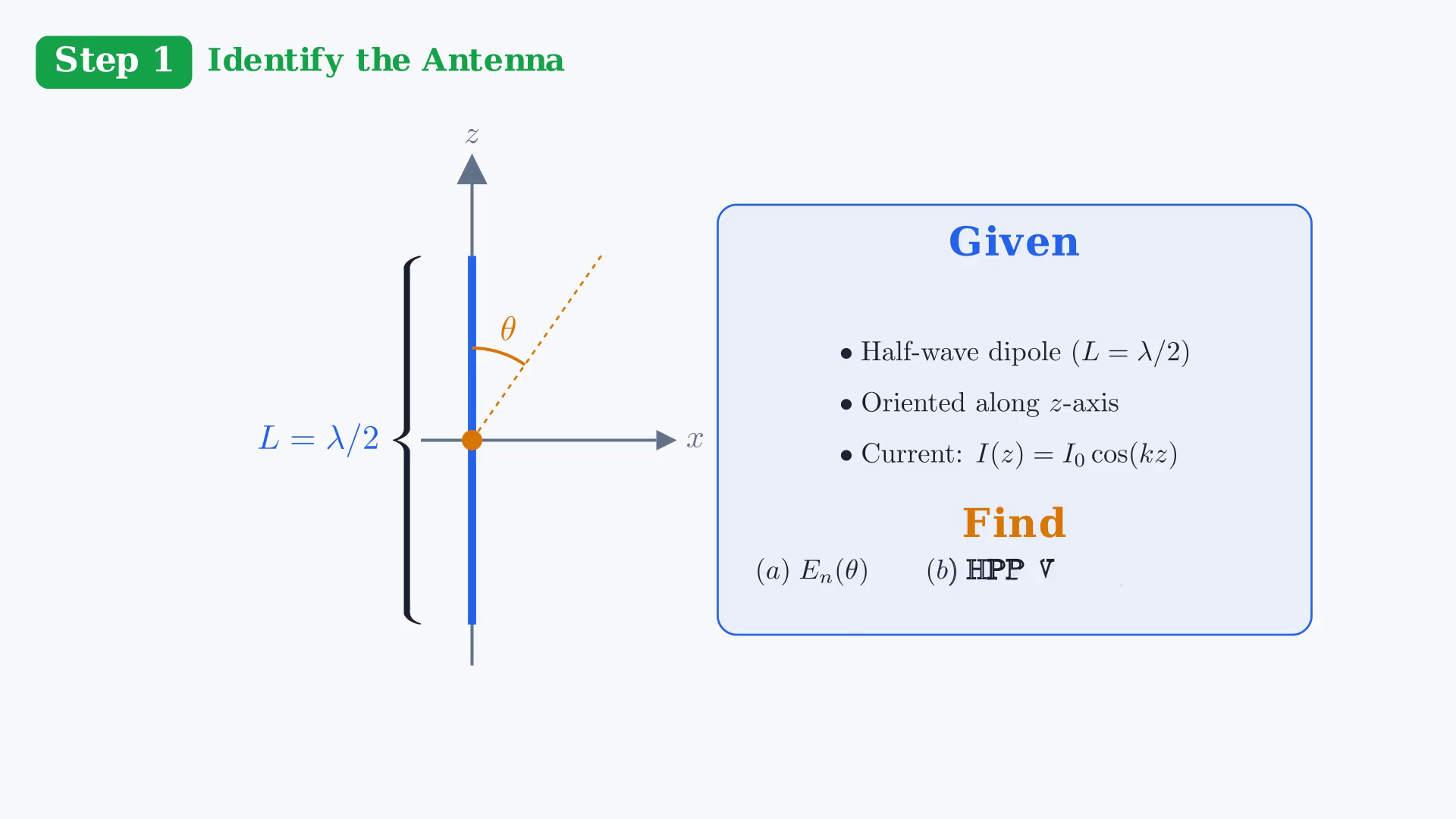
The same normalized field pattern determines the axial nulls, the 78-degree HPBW, and the 2.15 dBi directivity. Step one: identify the antenna.We have a half-wave dipole, so the total length equals λ/2.It sits along the z-axis, and the current distribution is cosine shaped: I(z)=I₀cos(kz).This is different from the short dipole where the current was roughly uniform.The cosine shape is what gives us the specific pattern we're about to calculate.Narration transcript
Step one: identify the antenna. We have a half-wave dipole, so the total length equals lambda over two. It sits along the z-axis, and the current distribution is cosine shaped: I of z equals I-zero times cosine of k-z. This is different from the short dipole where the current was roughly uniform. The cosine shape is what gives us the specific pattern we're about to calculate.
3. Normalize the far field to obtain the pattern
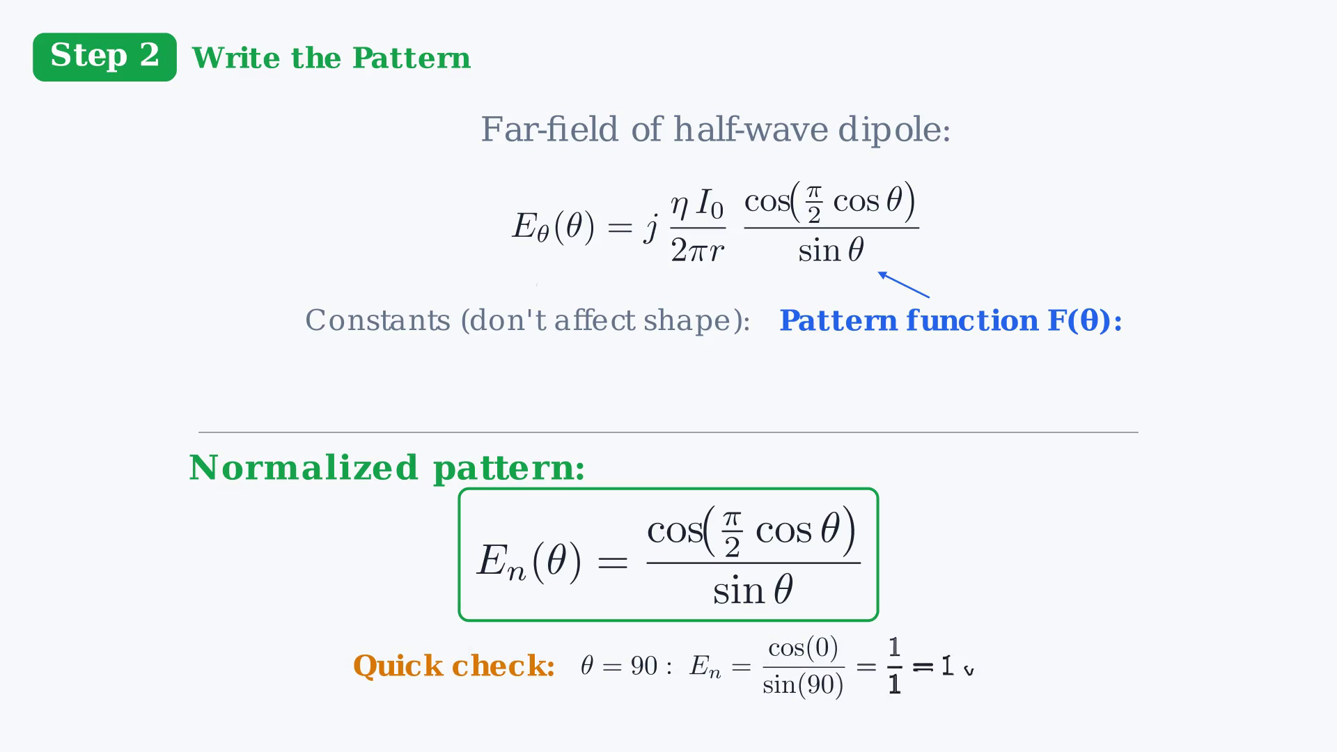
The same normalized field pattern determines the axial nulls, the 78-degree HPBW, and the 2.15 dBi directivity. Step two: write the far-field pattern.The full expression has constants like η, I₀, and 1/r that affect amplitude but not shape.The part that matters for the pattern is the numerator: cos[(π/2)cosθ]/sinθ.That's our normalized pattern Eₙ(θ).Quick sanity check: at θ=90°, cos0°=1 and sin90°=1, so Eₙ(90°)=1.The maximum is in the broadside direction.Good.Narration transcript
Step two: write the far-field pattern. The full expression has constants like eta, I-zero, and one-over-r that affect amplitude but not shape. The part that matters for the pattern is the numerator: cosine of pi-over-two times cosine-theta, divided by sine-theta. That's our normalized pattern E-n of theta. Quick sanity check: at theta equals ninety degrees, cosine of zero is one, sine of ninety is one, so E-n equals one. The maximum is in the broadside direction. Good.
4. Read the maximum and null directions from the pattern
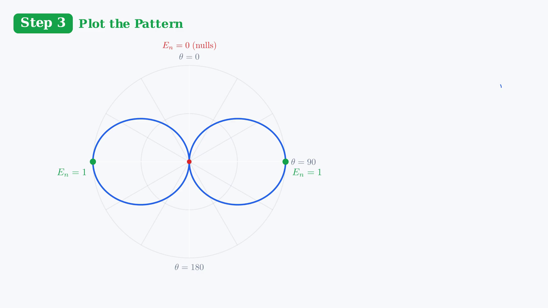
The same normalized field pattern determines the axial nulls, the 78-degree HPBW, and the 2.15 dBi directivity. Step three: let's plot it.The pattern looks like a figure eight in 2D, or a torus in 3D.The maximum is at θ=90°, perpendicular to the dipole.Nulls occur at θ=0° and 180°, that is along the dipole axis.If you compare this to a short dipole's sin² pattern, the half-wave dipole is slightly narrower.Not by much, but the directivity improvement is noticeable.Narration transcript
Step three: let's plot it. The pattern looks like a figure-eight in two-D, or a donut in three-D. The maximum is at theta equals ninety degrees, perpendicular to the dipole. Nulls occur at theta equals zero and one-eighty, that is along the dipole axis. If you compare this to a short dipole's sine-squared pattern, the half-wave dipole is slightly narrower. Not by much, but the directivity improvement is noticeable.
5. Solve the half-power angles and HPBW
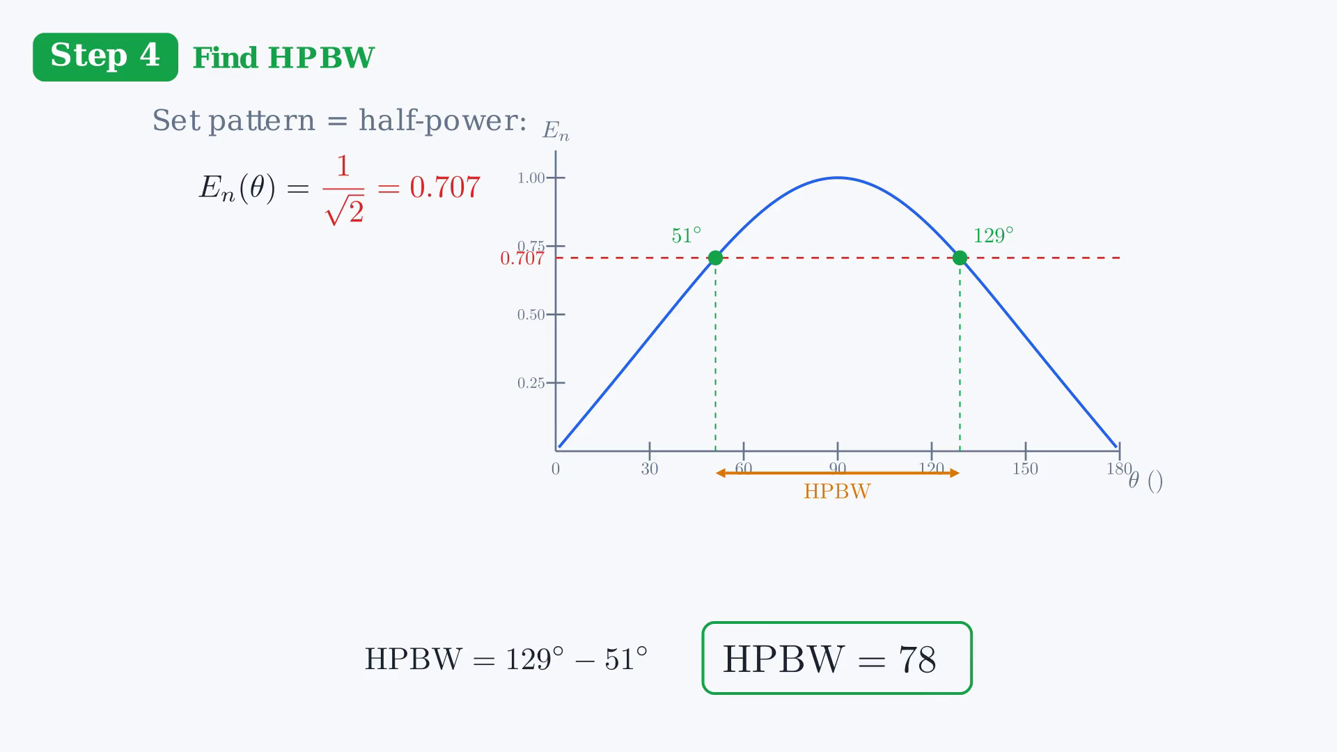
The same normalized field pattern determines the axial nulls, the 78-degree HPBW, and the 2.15 dBi directivity. Step four: find the HPBW.We set Eₙ(θ)= 1/√2, which is 0.707.This gives us a transcendental equation that we solve numerically.The two solutions are θ₁=51° and θ₂=129°.The half-power beamwidth is the difference:That's our answer for part b.Narration transcript
Step four: find the H-P-B-W. We set E-n of theta equal to one over root-two, which is zero-point-seven-oh-seven. This gives us a transcendental equation that we solve numerically. The two solutions are theta-one equals fifty-one degrees and theta-two equals one-hundred-twenty-nine degrees. The half-power beamwidth is the difference: one-twenty-nine minus fifty-one equals seventy-eight degrees. That's our answer for part b.
6. Calculate directivity in linear units and dBi
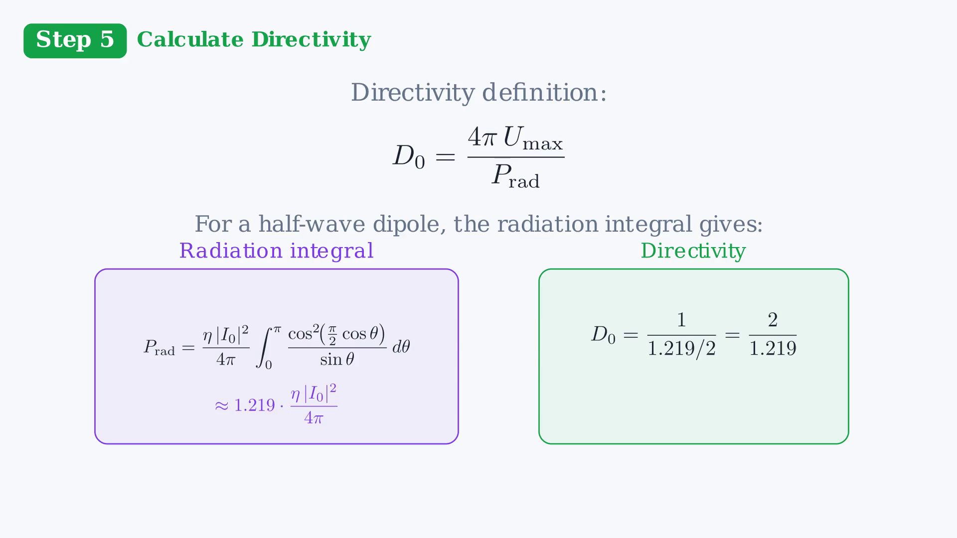
The same normalized field pattern determines the axial nulls, the 78-degree HPBW, and the 2.15 dBi directivity. Step five: calculate directivity.For the half-wave dipole, we need to evaluate a radiation integral.The radiation integral is ∫₀π F²(θ)sinθ dθ = 1.2188267 (about 1.219).Using the rounded integral gives 2/1.219≈1.6407; full precision and standard tables give D₀≈1.641–1.643.Converting to logarithmic units: 10log₁₀(D₀)≈2.15 dBi.That's part c done.Narration transcript
Step five: calculate directivity. D-zero equals four-pi times U-max divided by P-rad. For the half-wave dipole, we need to evaluate a radiation integral. The integral of cosine-squared-pi-over-two-cosine-theta divided by sine-theta, from zero to pi, gives approximately one-point-two-one-nine. Plugging in, D-zero equals two divided by one-point-two-one-nine, which is one-point-six-four-three. Converting to dBi: ten-log-ten of one-point-six-four-three equals two-point-one-five dBi. That's part c done.
7. Interpret the three-dimensional radiation pattern
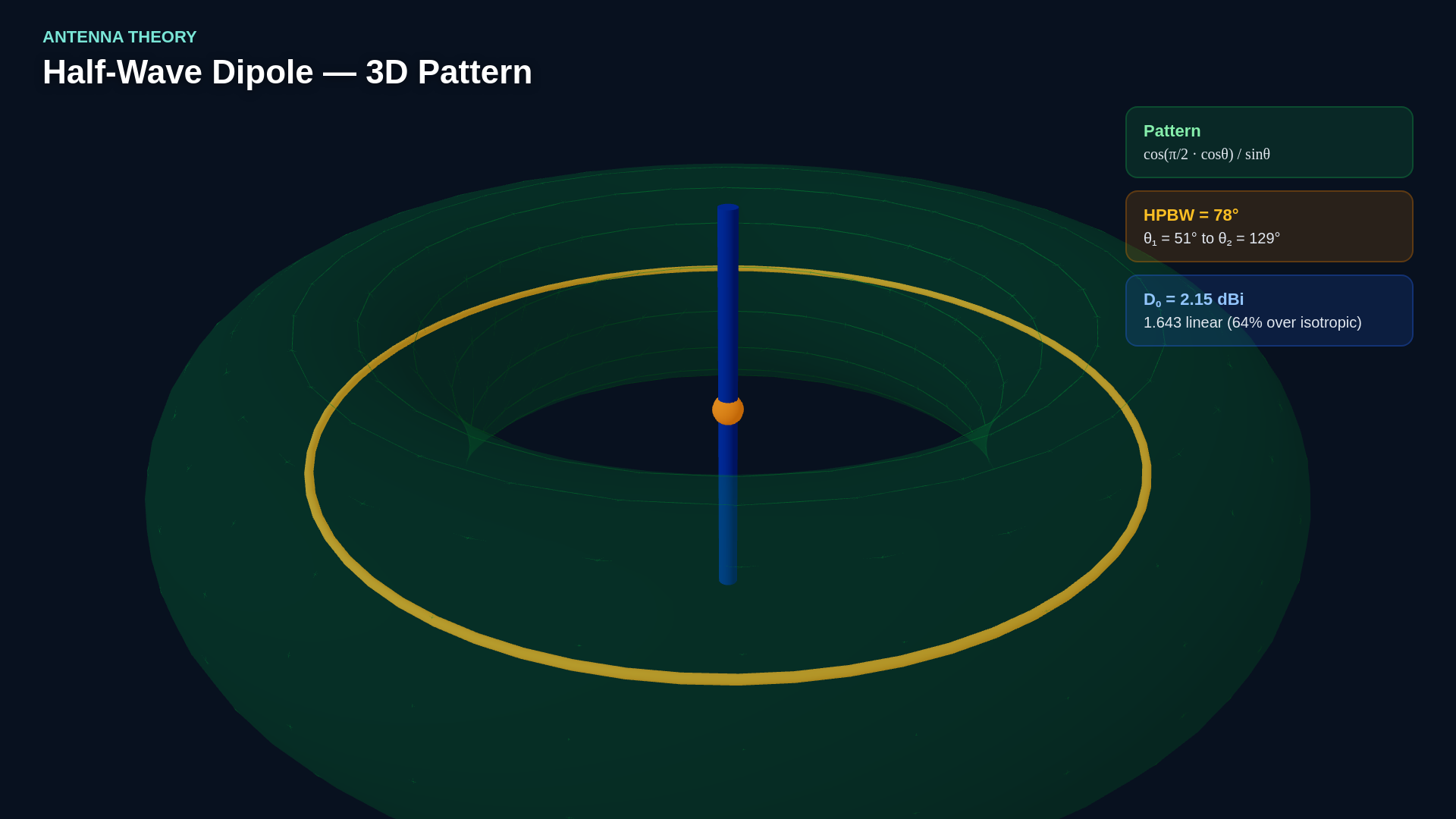
The same normalized field pattern determines the axial nulls, the 78-degree HPBW, and the 2.15 dBi directivity. Here's the 3D view of our half-wave dipole pattern.Notice the donut shape around the z-axis.The half-power beamwidth of 78° is marked, and the directivity of 2.15 dBi is modest but meaningful: about 64% more power density in the main direction compared to an isotropic radiator.Narration transcript
Here's the three-D view of our half-wave dipole pattern. Notice the donut shape around the z-axis. The half-power beamwidth of seventy-eight degrees is marked, and the directivity of two-point-one-five dBi is modest but meaningful: about sixty-four percent more power density in the main direction compared to an isotropic radiator.
8. Collect the results and limiting checks

The same normalized field pattern determines the axial nulls, the 78-degree HPBW, and the 2.15 dBi directivity. Let's box our answers.Part (a):Part (b): HPBW≈78°.Part (c): D₀≈1.64, or ≈2.15 dBi.These three numbers — pattern shape, beamwidth, and directivity — are the fingerprint of the half-wave dipole, and they appear in almost every antenna exam.Narration transcript
Let's box our answers. Part a: the normalized pattern is cosine of pi-over-two cosine-theta divided by sine-theta. Part b: H-P-B-W equals seventy-eight degrees. Part c: directivity equals one-point-six-four, or two-point-one-five dBi. These three numbers — pattern shape, beamwidth, and directivity — are the fingerprint of the half-wave dipole, and they appear in almost every antenna exam.
Source video: Antenna Theory #13 | Half-Wave Dipole Pattern & Directivity — Problem Solving 1 (4:25)