Antenna Theory · Half-Wave Dipole and the Reference Antenna

#10 The half-wave dipole's cosine current distribution, far-field integral, radiation pattern, directivity, and 73 Ω radiation resistance

Start from the realistic cosine current and derive the half-wave dipole's narrower pattern, 1.64 directivity, and 73 Ω reference value.

Question

Lesson frame showing the half-wave dipole's cosine current distribution, far-field integral, radiation pattern, and 73-ohm reference value. — Keeping the cosine current inside the integral produces the half-wave dipole's narrower pattern and practical reference values.

For a center-fed half-wave dipole, set up I(z′)=I₀cos(kz′); derive the cos[(π/2)cosθ]/sinθ far-field pattern and interpret its directivity and radiation resistance.

Written solution and narration transcript(shows the full solution)

Below are all the lines written in the notebook together with the full narration transcript.

1. Recall the short dipole's uniform-current assumption
Keeping the cosine current inside the integral produces the half-wave dipole's narrower pattern and practical reference values.
In lesson eight we solved the short dipole by treating the current as uniform along the wire.
That uniform current assumption made the integral trivial and gave us the sin(theta) pattern.
But a real antenna that is not electrically tiny cannot carry a constant current from feed to tip.
The current must go to zero at the open ends of the wire.
So the first upgrade is to replace the uniform current with a realistic distribution.
Narration transcript
In lesson eight we solved the short dipole by treating the current as uniform along the wire. That uniform current assumption made the integral trivial and gave us the sine theta pattern. But a real antenna that is not electrically tiny cannot carry a constant current from feed to tip. The current must go to zero at the open ends of the wire. So the first upgrade is to replace the uniform current with a realistic distribution.
2. Build the cosine standing-wave current on a λ/2 dipole
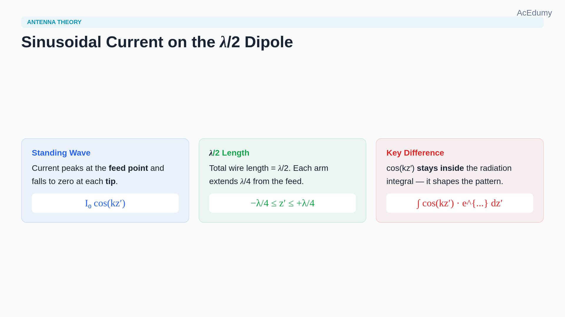
Keeping the cosine current inside the integral produces the half-wave dipole's narrower pattern and practical reference values.
On a center-fed dipole of total length l, the current follows a standing-wave shape.
It peaks at the feed point and drops to zero at each tip.
For a half-wave dipole, where the total length equals λ/2, the distribution is I₀ cos(kz′).
This cosine profile is the key difference from the short dipole.
Now the radiation integral no longer collapses to a constant times the wire length; the cosine current must stay inside the integral and shape the final pattern.
Narration transcript
On a center-fed dipole of total length l, the current follows a standing-wave shape. It peaks at the feed point and drops to zero at each tip. For a half-wave dipole, where the total length equals lambda over two, the distribution is I zero times cosine of k z prime. This cosine profile is the key difference from the short dipole. Now the radiation integral no longer collapses to a constant times the wire length; the cosine current must stay inside the integral and shape the final pattern.
3. Keep the varying current inside the far-field integral
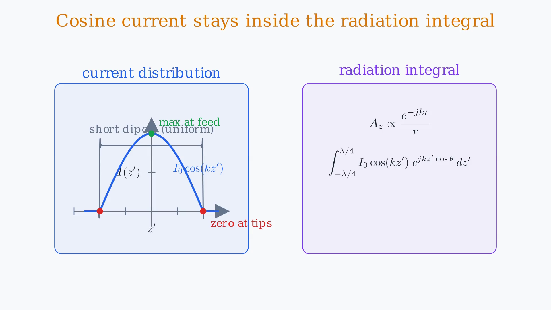
Keeping the cosine current inside the integral produces the half-wave dipole's narrower pattern and practical reference values.
Place the half-wave dipole symmetrically on the z axis, running from −λ/4 to +λ/4.
The far-field vector potential integral now reads: the same 1/r factor comes outside, but the integrand carries I₀ cos(kz′) times the source-dependent phase.
Unlike the short dipole, we cannot pull the current outside because it varies along the wire.
We evaluate the integral directly, and the result is a new pattern function.
Narration transcript
Place the half-wave dipole symmetrically on the z axis, running from minus lambda over four to plus lambda over four. The far-field vector potential integral now reads: the same one over r factor comes outside, but the integrand carries I zero cosine of k z prime times the source-dependent phase. Unlike the short dipole, we cannot pull the current outside because it varies along the wire. We evaluate the integral directly, and the result is a new pattern function.
4. Derive the cos[(π/2)cosθ]/sinθ pattern
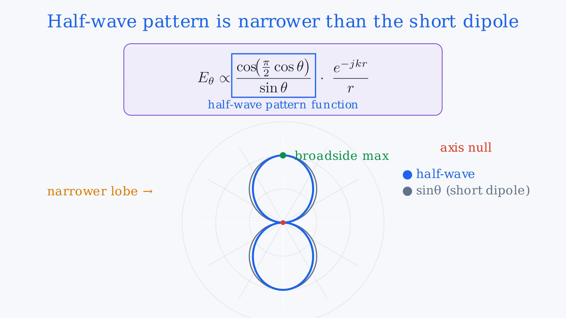
Keeping the cosine current inside the integral produces the half-wave dipole's narrower pattern and practical reference values.
After evaluating the integral, the far-field of the half-wave dipole becomes E_θ ∝ cos[(π/2)cosθ]/sinθ, times the usual 1/r decay.
Compare this with the short dipole's pure sin(theta).
Both patterns are zero on the axis and maximum at broadside, but the half-wave pattern is slightly narrower.
The extra cosine numerator squeezes the main lobe inward, concentrating slightly more power toward the equator.
Narration transcript
After evaluating the integral, the far-field of the half-wave dipole becomes E theta proportional to cosine of pi over two times cosine theta, divided by sine theta, times the usual one over r decay. Compare this with the short dipole's pure sine theta. Both patterns are zero on the axis and maximum at broadside, but the half-wave pattern is slightly narrower. The extra cosine numerator squeezes the main lobe inward, concentrating slightly more power toward the equator.
5. Interpret the narrower three-dimensional dipole pattern
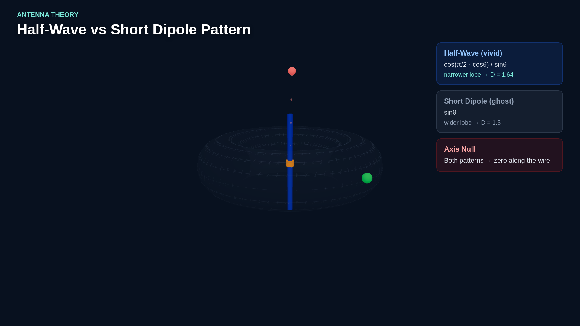
Keeping the cosine current inside the integral produces the half-wave dipole's narrower pattern and practical reference values.
In three dimensions this narrower pattern still looks like a doughnut around the dipole axis, but it is a thinner doughnut than the short dipole produces.
The null along the wire axis remains; that is a fundamental feature of any linear dipole.
The broadside maximum is still the strongest direction.
What has changed is that the half-wave dipole pushes a little more energy toward broadside, making it a slightly better radiator in the equatorial plane.
Narration transcript
In three dimensions this narrower pattern still looks like a doughnut around the dipole axis, but it is a thinner doughnut than the short dipole produces. The null along the wire axis remains; that is a fundamental feature of any linear dipole. The broadside maximum is still the strongest direction. What has changed is that the half-wave dipole pushes a little more energy toward broadside, making it a slightly better radiator in the equatorial plane.
6. Use the 1.64 directivity and 73 Ω radiation resistance
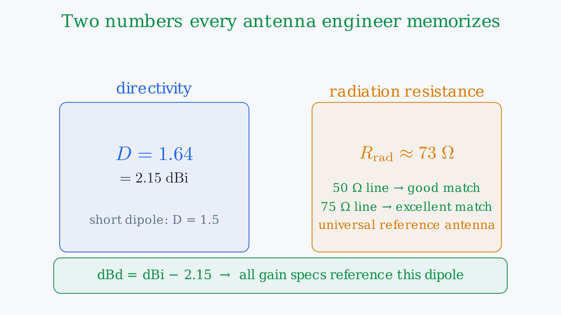
Keeping the cosine current inside the integral produces the half-wave dipole's narrower pattern and practical reference values.
The half-wave dipole gives us two numbers that every antenna engineer memorizes.
The directivity is 1.64, or about 2.15 dBi.
And the radiation resistance at the feed point is approximately 73 Ω.
That 73 Ω value is remarkably close to standard transmission line impedances of 50 and 75 Ω.
This near match is the practical reason why the half-wave dipole became the universal reference antenna.
Almost every antenna gain specification you encounter is measured relative to this dipole.
Narration transcript
The half-wave dipole gives us two numbers that every antenna engineer memorizes. The directivity is one point six four, or about two point one five d B i. And the radiation resistance at the feed point is approximately seventy-three ohms. That seventy-three ohm value is remarkably close to standard transmission line impedances of fifty and seventy-five ohms. This near match is the practical reason why the half-wave dipole became the universal reference antenna. Almost every antenna gain specification you encounter is measured relative to this dipole.
7. Summarize three upgrades from short to half-wave
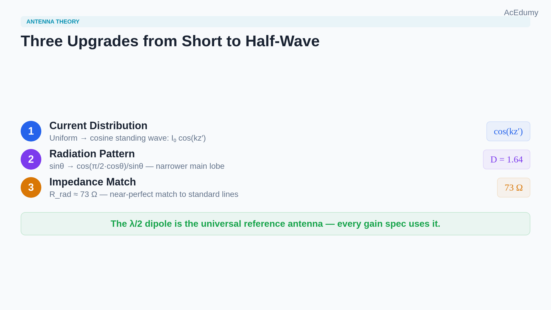
Keeping the cosine current inside the integral produces the half-wave dipole's narrower pattern and practical reference values.
The half-wave dipole upgrades the short dipole in three ways.
First, the current distribution changes from uniform to cosine, reflecting the standing wave on a real wire.
Second, the radiation pattern narrows from sin(theta) to cos[(π/2)cosθ]/sinθ, giving slightly higher directivity.
Third, the radiation resistance of 73 Ω makes impedance matching straightforward, which is why this antenna became the standard reference.
Narration transcript
The half-wave dipole upgrades the short dipole in three ways. First, the current distribution changes from uniform to cosine, reflecting the standing wave on a real wire. Second, the radiation pattern narrows from sine theta to the cosine over sine function, giving slightly higher directivity. Third, the radiation resistance of seventy-three ohms makes impedance matching straightforward, which is why this antenna became the standard reference.
8. Bridge from a single element to antenna arrays
Keeping the cosine current inside the integral produces the half-wave dipole's narrower pattern and practical reference values.
So far every antenna we have studied is a single element.
The next natural step is to ask what happens when we combine multiple dipoles into an array.
That combination introduces a new degree of freedom: the spacing and phasing between elements can steer the beam electronically without moving the antenna.
That is the doorway to array theory.
Narration transcript
So far every antenna we have studied is a single element. The next natural step is to ask what happens when we combine multiple dipoles into an array. That combination introduces a new degree of freedom: the spacing and phasing between elements can steer the beam electronically without moving the antenna. That is the doorway to array theory.