Circuit Theory 2 · Low-pass and high-pass filters

#21 Unloaded RC filters, normalized corner, positive-frequency phase, design and loading

Compare RC low-pass and high-pass voltage responses with readable fractions, explicit phase limits, cutoff units and loading assumptions.

Question

Reviewed original English video reference comparing RC filter topology, response, cutoff or design. — Reference from the existing video. The same-corner and Bode roles use summary and introduction cards from the same final; complete formulas and loading assumptions are stated in the notebook.

Compare ideal real linear time-invariant first-order RC voltage filters with constant positive R and C, zero initial state, ideal zero-output-resistance voltage drive and no output load. Low-pass uses a series R and a shunt C to the common reference, with output measured across C. For a ground-referenced high-pass output use a series C and a shunt R to reference, with output across R. Merely moving a probe to the original input node is not a high-pass transformation; explicitly specify both output terminals and preserve the input/reference wiring. With τ=RC, H_LP(s)=1/(1+sτ), H_HP(s)=sτ/(1+sτ). Both have a stable pole−1/τ; their causal regions include the imaginary axis. H_HP has a zero at the origin. These are sinusoidal steady-state responses, not full switched-on transients. For ω>0, H_LP(jω)=1/(1+jωτ), H_HP(jω)=jωτ/(1+jωτ). Magnitudes are1/sqrt(1+(ωτ)^2) and ωτ/sqrt(1+(ωτ)^2). Their complex sum is one, and their squared magnitudes sum to one; their magnitudes do not sum to one. The sum identity assumes the same ideal time constant and chosen consistent voltage references, not arbitrary loaded independent filters. Low-pass tends to unity at DC and zero at high frequency; high-pass tends to zero at DC and unity at high frequency. Its phase at exactly zero gain is undefined; its positive-frequency phase limit at DC is+90degrees, not a phase assigned to a nonzero DC output. In radians φ_LP=−atan(ωτ), φ_HP=π/2−atan(ωτ). Their phase difference at each positive frequency is90degrees; they are opposite at the corner only, not negatives of each other at all frequencies. The source graphic's mirrored-phase phrase is qualitative. The common angular corner is ω_c=1/(RC), and ordinary cutoff f_c=1/(2πRC), with ω=2πf. At the corner, both magnitudes are1/sqrt2 relative to their unity passband gains and G_c=20log10(1/sqrt2)≈−3.0103dB. The original generic first-order-passive wording must be qualified: for a loaded filter, normalize to its actual passband gain rather than assuming absolute0.707. Calling an amplitude ratio half power requires appropriate equal real resistance references; a reactive unloaded output alone does not establish power transfer. The cutoff is not a hard wall. Exact logarithmic slopes are−20(ωτ)^2/(1+(ωτ)^2) for LP and20/(1+(ωτ)^2) for HP in dB per decade. At the corner these are−10 and+10;±20 are remote asymptotes. For the ideal design example f_c=1000Hz,C=100nF=1e−7F gives R=1/(2πf_cC)=1591.54943ohms≈1.59kΩ. This is a calculated nominal value, not a claim that rounding or component tolerance leaves cutoff unchanged. Recalculate after selecting standard parts; no purchasing or hardware changes are performed. Source and load resistance can alter both passband gain and corner. For LP with source resistance R_s, series filter R and positive resistive load R_L parallel to C, set R_t=R+R_s. DC gain is R_L/(R_t+R_L) and time constant is C(R_t parallel R_L). For HP with R_e=(R parallel R_L), the source resistance is in series with C and the output equivalent resistance; high-frequency gain is R_e/(R_s+R_e), time constant C(R_s+R_e). Suitable input/output buffers isolate those loading effects within their bandwidth and operating limits; buffering does not abolish component tolerances. All ten original final frames were individually reviewed. The same-corner frame includes an unqualified half-power statement, so that notebook role uses the same final's summary frame. The Bode comparison frame has inconsistent numeric y-tick positions relative to its generated curves, so that role uses the same final's introductory comparison card. No new graphic or source video was generated. Retained circuit drawings have minor C/plate-label overlap but clear connected RC topologies. The filter-idea colored bars are an illustrative signal spectrum, not the analytic filter response. The phase endpoint ticks are qualitative; the design card's second small instruction touches a box edge but remains visible. The final card's next-topic wording is broader than the original narration; original say is authoritative. Legacy one-line fractions, raw LP/HP labels and omega/tau text remain manual visual/teaching-QA caveats; the notebook uses the existing common renderer with explicit grouped subscripts and denominators. Original say, all ten MP3s and all45 aligned cue boundaries remain unchanged. Cached-large ASR recognized1kHz,100nF,1.59kOhms and±45degree signs; FCC/RC/FC and cue-for-Q are tokenization observations, not confirmed numeric or sign errors. No alignment override,prompt or threshold modification. This remains an unpublished draft,not full human listening,complete motion QA or publication approval.

Written solution and narration transcript(shows the full solution)

Below are all the lines written in the notebook together with the full narration transcript.

1. Choose the output and frequency band
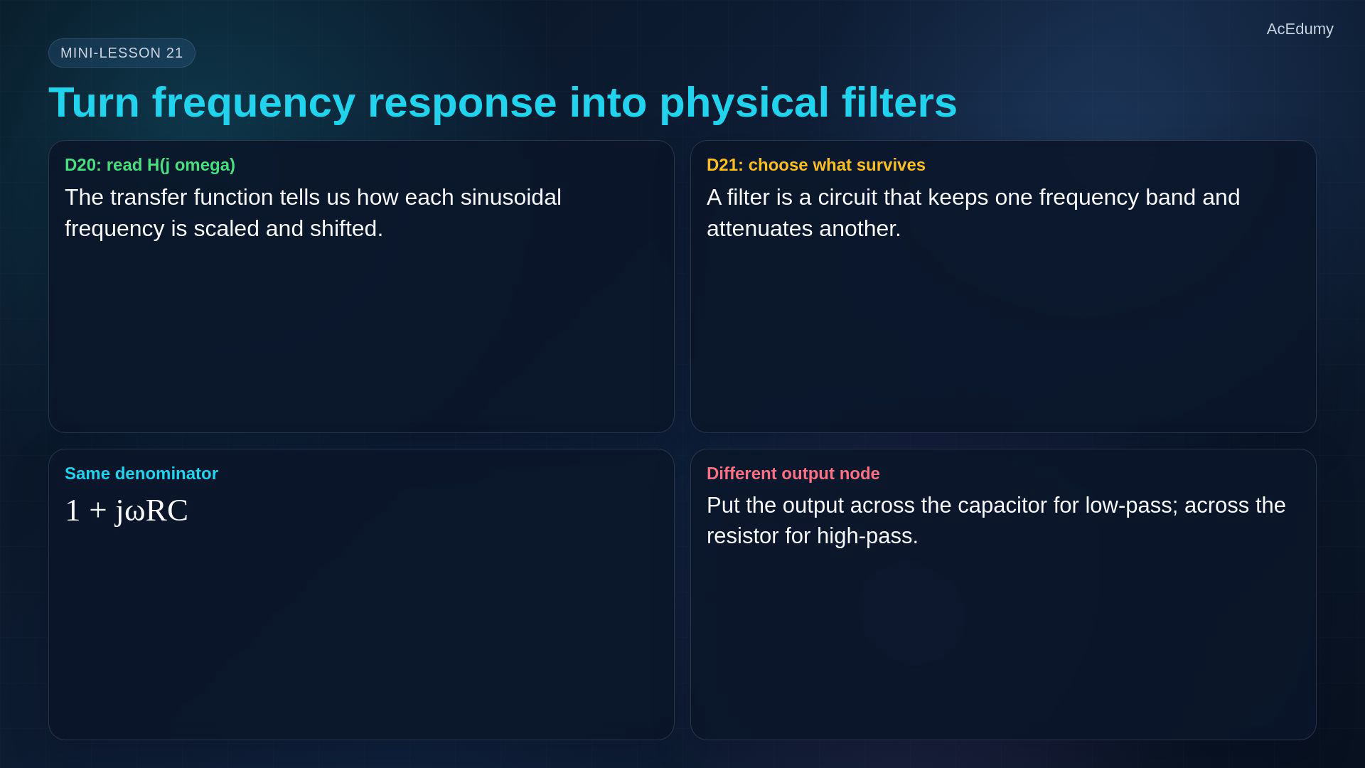
Reference from the existing video. The same-corner and Bode roles use summary and introduction cards from the same final; complete formulas and loading assumptions are stated in the notebook.
Use the stable, initially relaxed input-output frequency-response description from lesson 20.
Compare two ideal RC voltage filters with the same positive R and C.
The low-pass preserves low-frequency voltage and attenuates high frequencies.
The high-pass attenuates low frequencies and approaches unity gain at high frequency.
Choose the output across C or R; grounded versions require the corresponding component arrangement.
Narration transcript
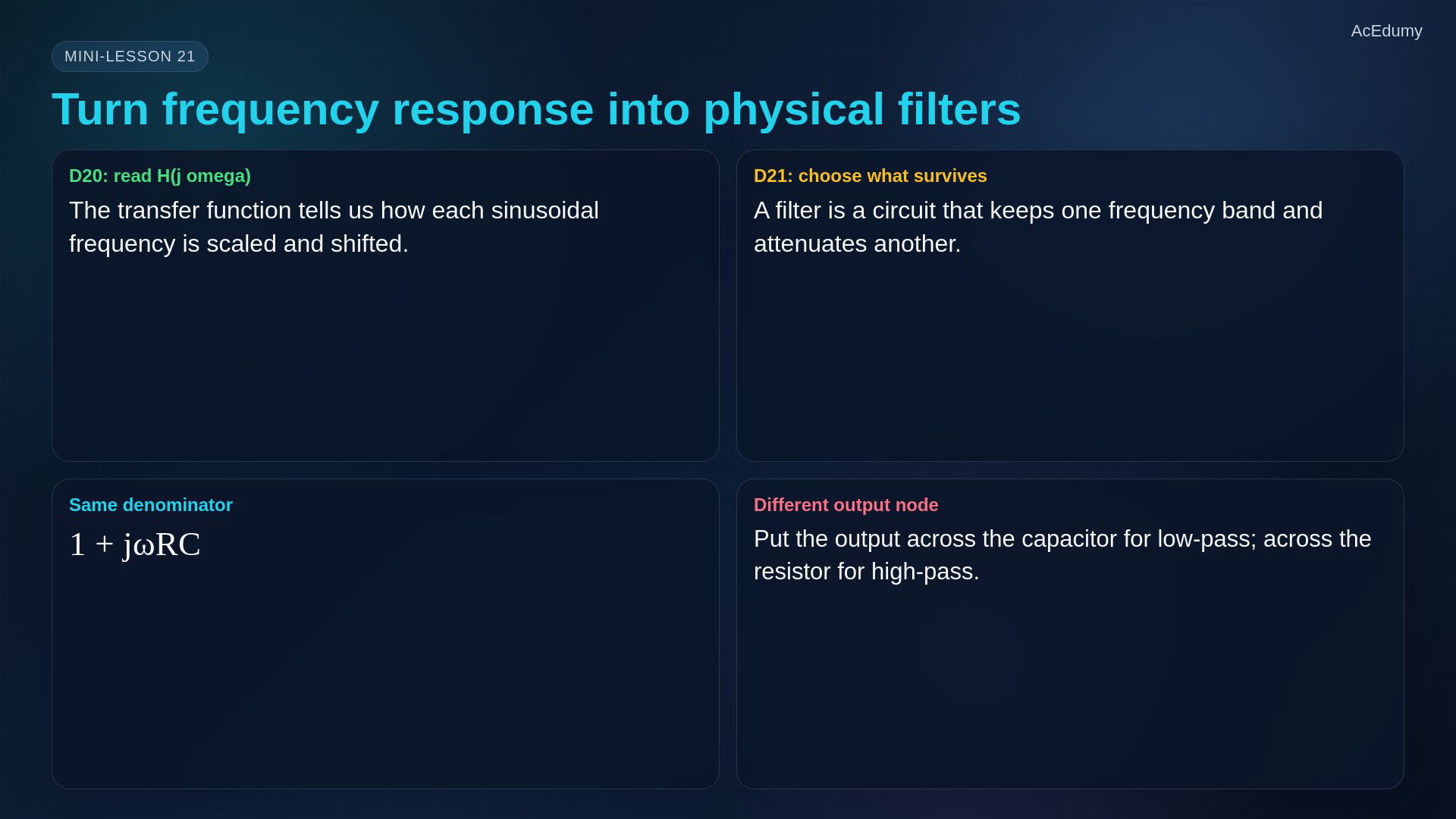
In the previous lesson, frequency response told us how a circuit treats each sinusoidal frequency. Now we turn that language into two physical circuits. A low-pass filter keeps the low-frequency part and reduces the high-frequency part. A high-pass filter does the opposite. Same resistor and capacitor idea, same corner frequency, but a different output node.
2. Define the normalized cutoff without a hard wall
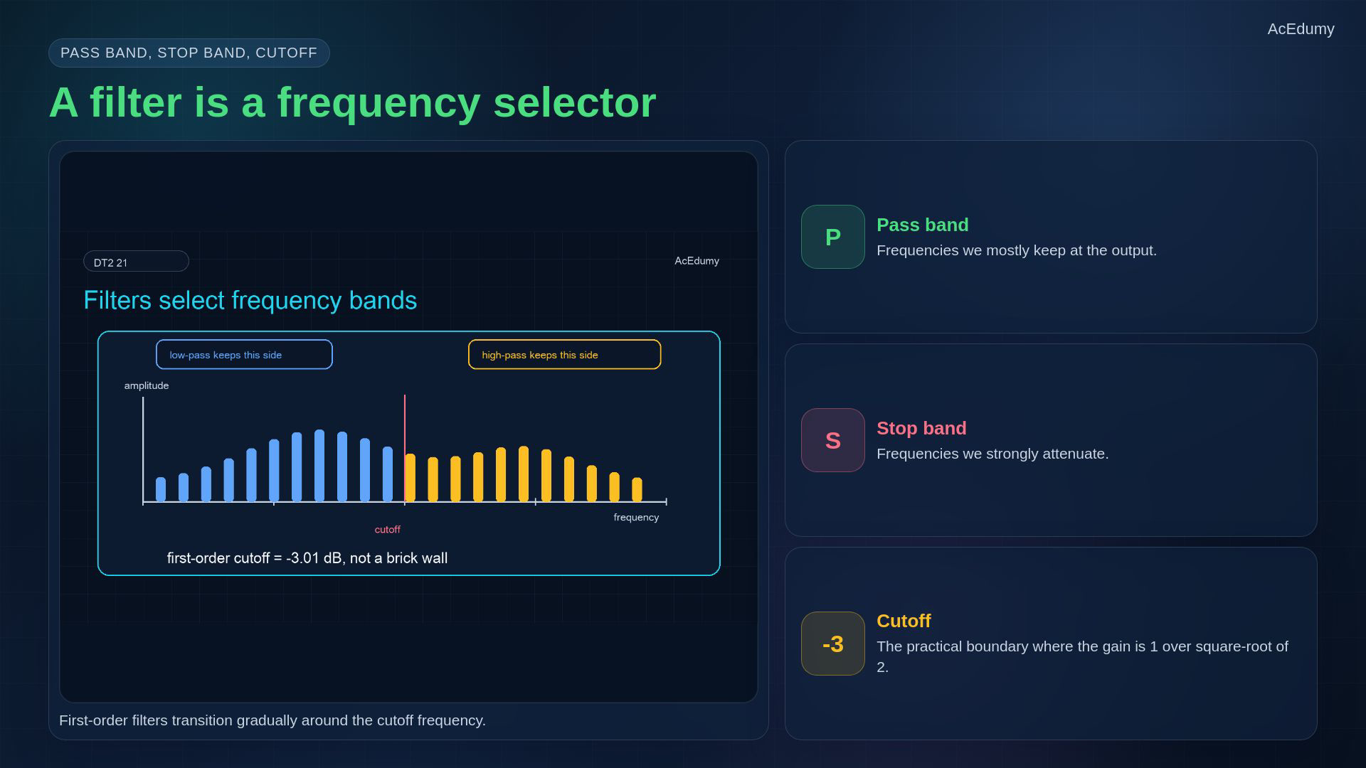
Reference from the existing video. The same-corner and Bode roles use summary and introduction cards from the same final; complete formulas and loading assumptions are stated in the notebook.
A filter selects frequency regions rather than individual time instants.
The pass band is the region intended to retain the signal.
The stop band is the region intended to attenuate it.
For these unity-passband first-order RC filters, the corner magnitude is:
$\displaystyle |H\left(j\omega _{c}\right)|=\frac{1}{\sqrt{2}}$
Narration transcript
Think of a filter as a frequency selector. The pass band is the region we want to keep. The stop band is the region we want to suppress. The cutoff frequency is not a hard wall; for a first-order passive filter it is the minus-three-decibel point, where the amplitude is one over square root of two.
3. Measure the unloaded output across the capacitor
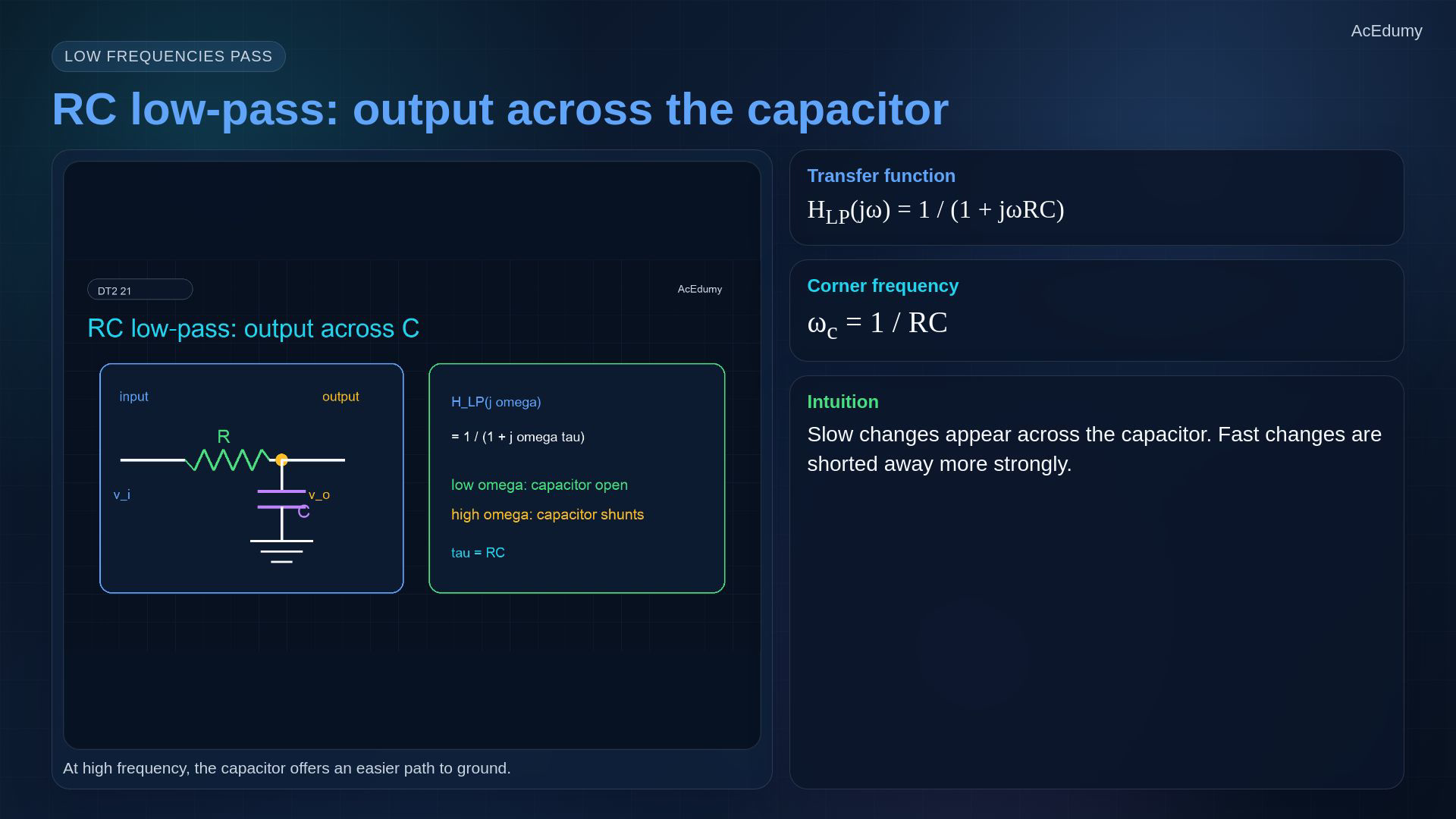
Reference from the existing video. The same-corner and Bode roles use summary and introduction cards from the same final; complete formulas and loading assumptions are stated in the notebook.
Low-pass: take the output voltage across the capacitor.
Use a series resistor and a capacitor from the output node to the common reference; assume no loading.
Well below the corner, the capacitor's impedance is large and the output approaches the input.
Well above the corner, the capacitor shunts the output more strongly.
With the stated voltage references:
$\displaystyle H_{\mathrm{LP}}\left(j\omega \right)=\frac{1}{1+j\omega \tau }$
Narration transcript
Start with the RC low-pass. Put the resistor in series, put the capacitor to ground, and measure the output across the capacitor. At low frequency, the capacitor is almost open, so very little current flows and the output is close to the input. At high frequency, the capacitor becomes an easy path to ground, so the output node is pulled down. The result is H low-pass of j omega equals one over one plus j omega tau.
4. Measure the output across the grounded resistor
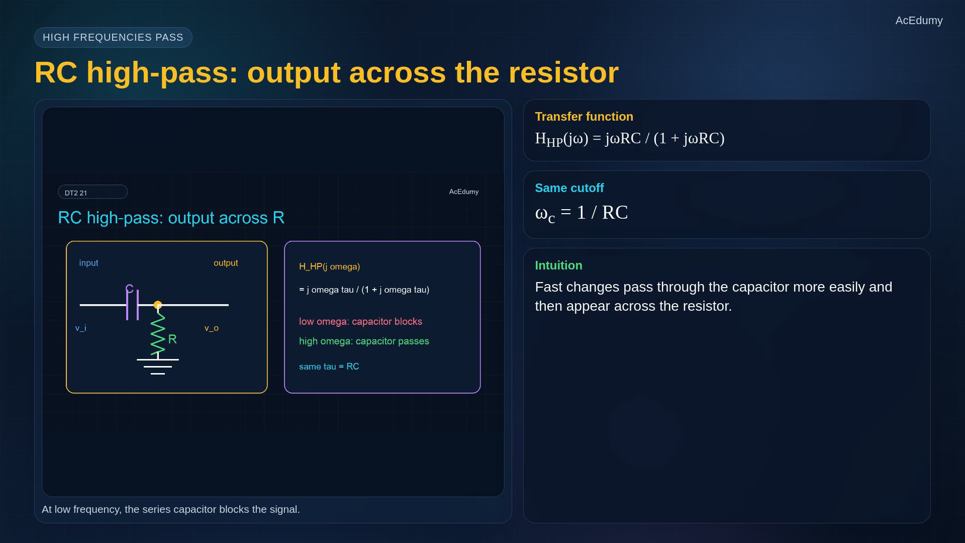
Reference from the existing video. The same-corner and Bode roles use summary and introduction cards from the same final; complete formulas and loading assumptions are stated in the notebook.
For a grounded high-pass output, use a series capacitor followed by a resistor to the common reference.
Measure the output across that resistor, not across the capacitor.
At low positive frequency the series capacitor has large impedance; at DC it blocks steady current.
At high frequency its impedance becomes small relative to R, so the output approaches the input.
The corresponding high-pass transfer is:
$\displaystyle H_{\mathrm{HP}}\left(j\omega \right)=\frac{j\omega \tau }{1+j\omega \tau }$
Narration transcript
Now move the output to the resistor side after a series capacitor. This is the RC high-pass. At low frequency, the capacitor blocks change, so the output across the resistor is small. At high frequency, the capacitor behaves almost like a short, so the input reaches the resistor and the output approaches the input. Its transfer function is j omega tau over one plus j omega tau.
5. Keep angular and ordinary cutoff frequencies distinct
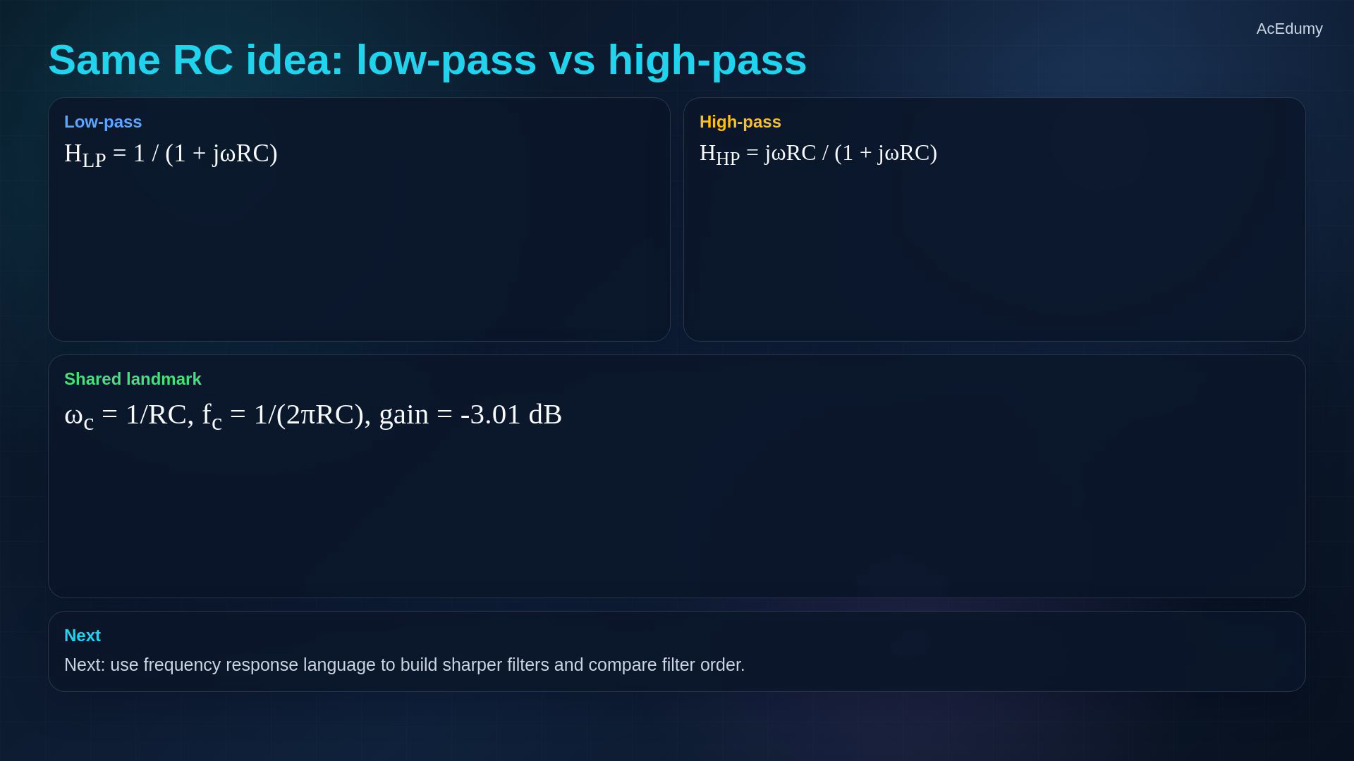
Reference from the existing video. The same-corner and Bode roles use summary and introduction cards from the same final; complete formulas and loading assumptions are stated in the notebook.
For the ideal unloaded pair with the same component values:
$\displaystyle \tau =R C$
Keep radians per second and hertz distinct:
$\displaystyle \omega _{c}=\frac{1}{\tau }, f_{c}=\frac{1}{2\pi R C}$
Both corner magnitudes are equal; the numerical amplitude gain in decibels is:
$\displaystyle |H\left(j\omega _{c}\right)|=\frac{1}{\sqrt{2}}, G_{c}\approx -3.0103$
At the positive corner frequency, in degrees:
$\displaystyle \varphi _{\mathrm{LP}}\left(\omega _{c}\right)=-45^{\circ}, \varphi _{\mathrm{HP}}\left(\omega _{c}\right)=45^{\circ}$
Narration transcript
Both circuits share the same time constant tau equals R C. The corner angular frequency is omega c equals one over tau, and the ordinary cutoff frequency is f c equals one over two pi R C. At that corner, both magnitudes are one over square root of two, which is minus three point zero one decibels. The low-pass phase is minus forty-five degrees, while the high-pass phase is plus forty-five degrees.
6. Compare exact curves and asymptotic slopes
Reference from the existing video. The same-corner and Bode roles use summary and introduction cards from the same final; complete formulas and loading assumptions are stated in the notebook.
For equal time constants the complex responses are complementary, not their magnitudes:
$\displaystyle H_{\mathrm{LP}}\left(j\omega \right)+H_{\mathrm{HP}}\left(j\omega \right)=1$
Low-pass gain tends to zero decibels well below cutoff; its slope tends to minus twenty decibels per decade far above cutoff.
High-pass gain rises at approximately plus twenty decibels per decade far below cutoff and tends to zero decibels far above it.
Narration transcript
On the Bode magnitude plot, the two curves are complementary. The low-pass starts near zero decibels and then rolls off at about minus twenty decibels per decade after the corner. The high-pass starts very small, rises at about plus twenty decibels per decade before the corner, and then flattens near zero decibels.
7. Read positive-frequency lead and lag
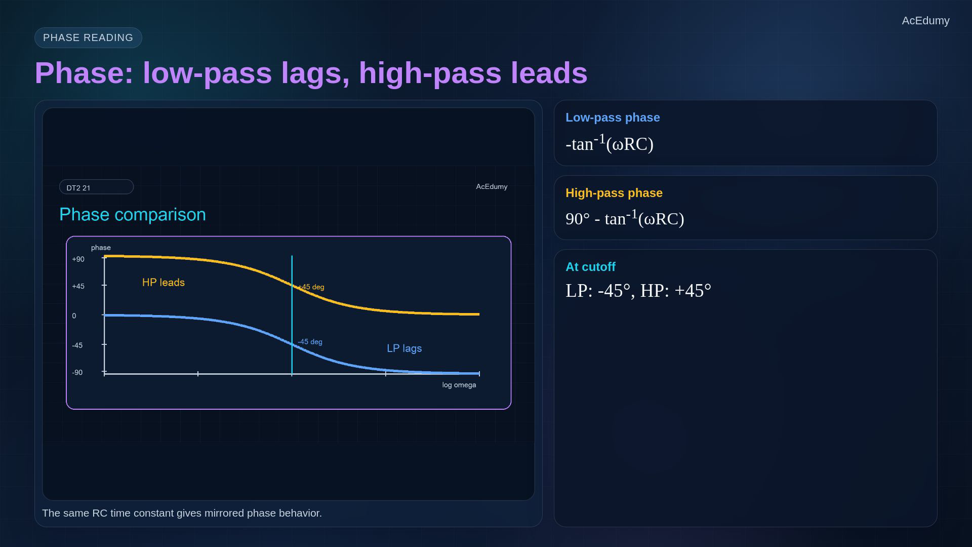
Reference from the existing video. The same-corner and Bode roles use summary and introduction cards from the same final; complete formulas and loading assumptions are stated in the notebook.
Read phase at positive frequencies where the gain is nonzero.
Low-pass phase in radians:
$\displaystyle \varphi _{\mathrm{LP}}\left(\omega \right)=-\arctan \left(\omega \tau \right)$
High-pass phase in radians for positive frequency:
$\displaystyle \varphi _{\mathrm{HP}}\left(\omega \right)=\frac{\pi }{2}-\arctan \left(\omega \tau \right)$
The two phases are opposite only at the corner; there they are minus and plus forty-five degrees.
Narration transcript
The phase plots tell the same story in another language. The low-pass starts near zero degrees and approaches minus ninety degrees as frequency increases. The high-pass starts near plus ninety degrees and approaches zero degrees as frequency increases. At the corner, the phase values are symmetric: minus forty-five and plus forty-five degrees.
8. Calculate a resistor from the target cutoff
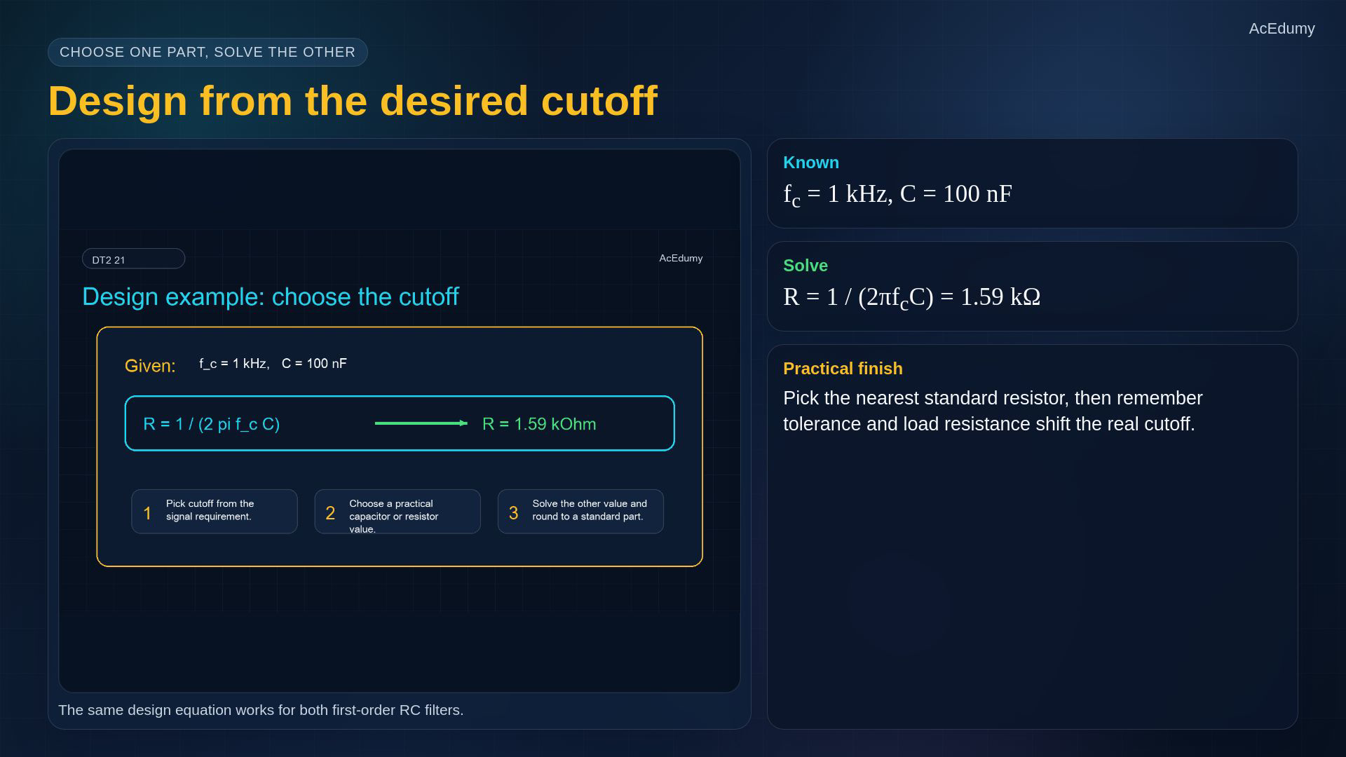
Reference from the existing video. The same-corner and Bode roles use summary and introduction cards from the same final; complete formulas and loading assumptions are stated in the notebook.
Choose an ideal first-order RC design target before accounting for loading and tolerance.
Select the cutoff and one component, then solve for the other.
For a one-kilohertz target and a 100-nanofarad capacitor:
$\displaystyle R=\frac{1}{2\pi f_{c} C}$
The ideal calculated resistance is approximately:
$\displaystyle R\approx 1591.55\left[\mathrm{Ω}\right]$
Choose a suitable standard value and recalculate the actual cutoff, including tolerances and source/load effects.
Narration transcript
A first-order RC filter is easy to design. Choose the cutoff frequency, choose either R or C, and solve for the other one. For example, if f c is one kilohertz and C is one hundred nanofarads, then R equals one over two pi f c C. That gives about one point five nine kilo-ohms. In practice you choose the nearest standard resistor value.
9. Check output references and source or load resistance
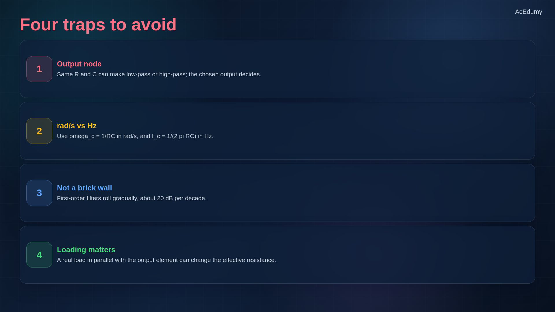
Reference from the existing video. The same-corner and Bode roles use summary and introduction cards from the same final; complete formulas and loading assumptions are stated in the notebook.
Four checks before treating the ideal result as a practical filter.
State both output terminals and the common reference; swapping a grounded topology is not merely relabelling a node.
Do not omit the full reciprocal denominator or the factor of pi:
$\displaystyle \omega _{c}=\frac{1}{R C}, f_{c}=\frac{1}{2\pi R C}$
The transition is gradual; the quoted twenty-decibel slopes are asymptotic, not an ideal frequency wall.
Finite source and load resistance can change the passband gain and cutoff; suitable buffers isolate those loading effects.
Narration transcript
Four traps to avoid. First, the output node decides whether the same RC pair is low-pass or high-pass. Second, omega c equals one over R C, but f c equals one over two pi R C. Third, passive first-order filters are gradual; the cutoff is not an ideal brick wall. Fourth, real source and load resistance can shift the cutoff unless the filter is buffered.
10. Compare the two first-order RC responses
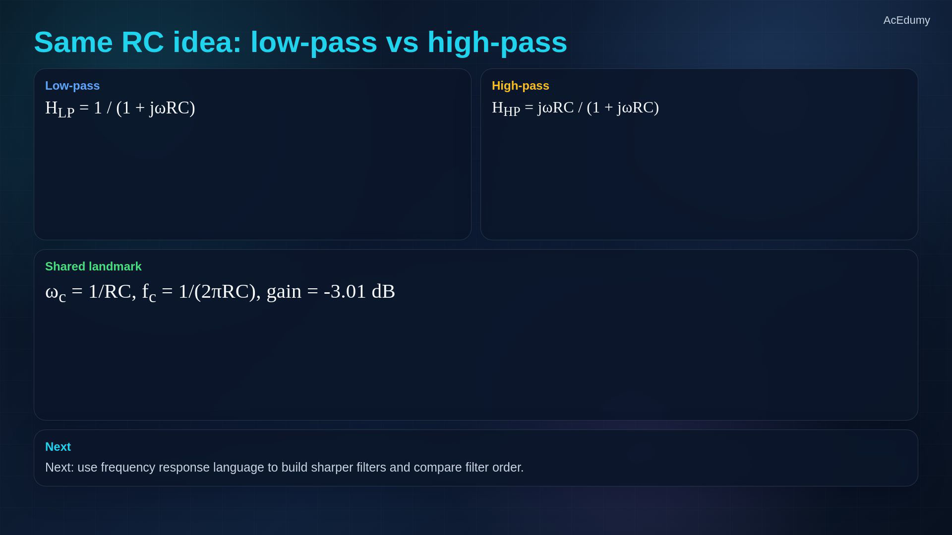
Reference from the existing video. The same-corner and Bode roles use summary and introduction cards from the same final; complete formulas and loading assumptions are stated in the notebook.
Summary: two first-order filters, one time constant.
Both use the same stable frequency-response framework.
For the ideal unloaded RC examples, the corner uses:
$\displaystyle \tau =R C, f_{c}=\frac{1}{2\pi R C}, G_{c}\approx -3.0103$
Across C gives low-pass; across R gives high-pass with the stated topology and voltage references.
Next: add another energy-storage element and study band-pass behavior, resonance and Q.
Narration transcript
Summary. Low-pass and high-pass filters are frequency selectors built from the same frequency-response idea. For first-order RC filters, tau equals R C, the cutoff is one over two pi R C, and the cutoff gain is minus three decibels. Changing the output node changes which side of the spectrum is kept. Next we add a second energy storage element and meet band-pass behavior, resonance, and Q.