#23 Magnetic boundary conditions and field-line refraction, flux linkage and inductance, magnetic energy and energy density

Below are all the lines written in the notebook together with the full narration transcript.

1. 1. Identify the final three pieces of statics

   

   We've covered a lot.

   The magnetic field H from Biot-Savart and Ampère.

   The flux density B, the no-monopole law, and all four Maxwell equations in static form.

   The Lorentz force, the torque on loops, and how materials respond through the relative permeability.

   Today closes the static electromagnetic block with three final pieces: how fields behave at the interface between two different materials, how we measure a coil's ability to store magnetic flux through its inductance, and where the magnetic energy lives.

   Narration transcript

   We've covered a lot. The magnetic field H from Biot-Savart and Ampère. The flux density B, the no-monopole law, and all four Maxwell equations in static form. The Lorentz force, the torque on loops, and how materials respond through the relative permeability. Today closes the static electromagnetic block with three final pieces: how fields behave at the interface between two different materials, how we measure a coil's ability to store magnetic flux through its inductance, and where the magnetic energy lives.

2. 2. Derive normal-B and tangential-H conditions

   

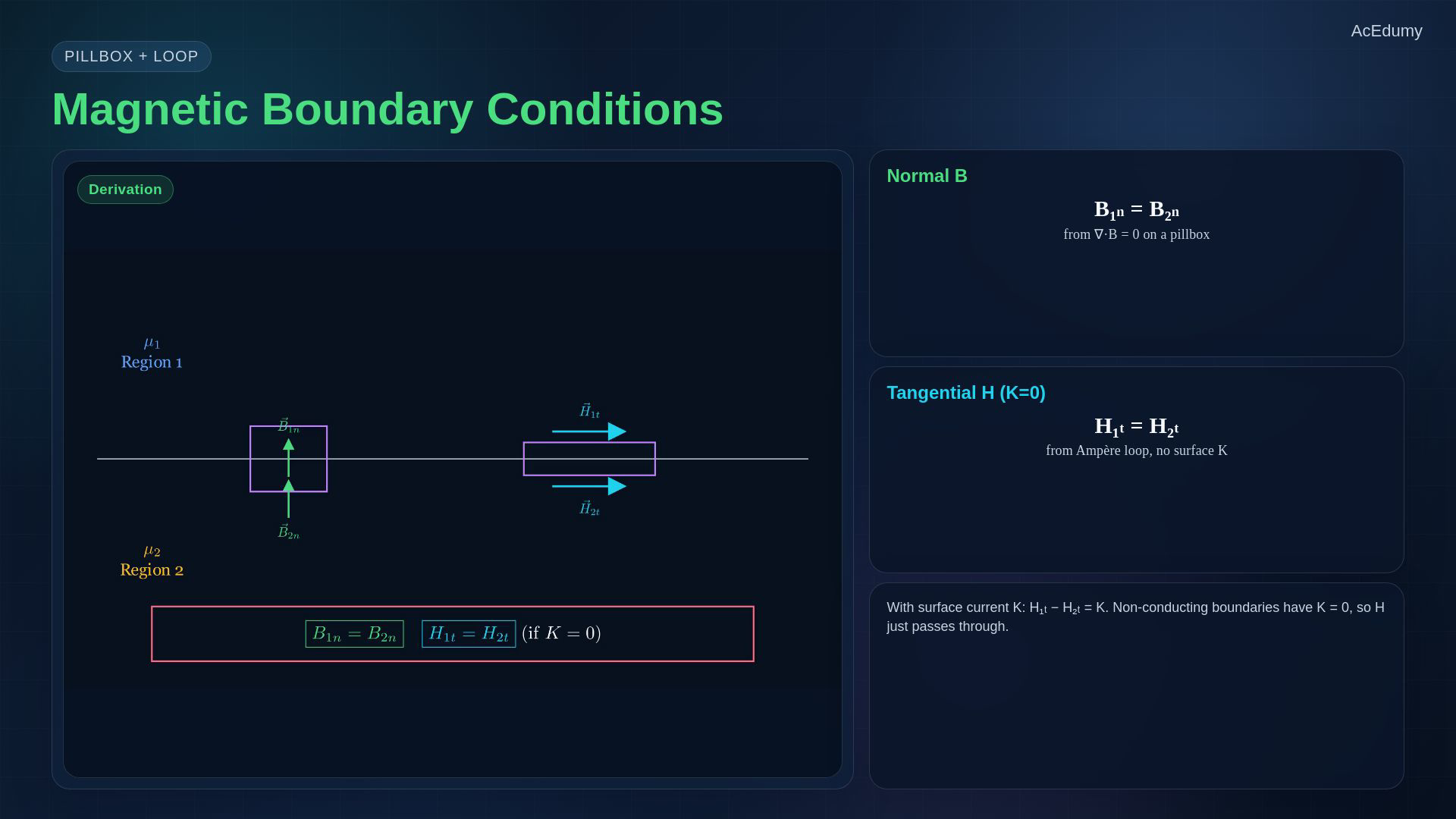
   Imagine two materials stacked on top of each other, with permeabilities μ₁ and μ₂.

   A magnetic field crosses the interface.

   What does it look like on the other side?

   Start with the normal component of B and ∮_S B·dS = 0.

   Apply divergence of B equals zero in integral form to a pillbox straddling the interface.

   Why a pillbox?

   Because we want to turn the volume equation into a surface one — the pillbox is a tiny cylindrical volume with top and bottom on opposite sides of the interface, and its side walls shrink to zero as the box flattens.

   In that limit, only the top and bottom contribute, and no flux can leave or enter.

   Flux continuity gives B₁ₙ = B₂ₙ.

   Normal B is continuous.

   Now the tangential component of H.

   Apply Ampère's circuit law to a thin rectangular loop straddling the interface, with its long sides parallel to the surface.

   Why this loop?

   Because as the short sides shrink, only the long sides matter, and the integral reduces to H₁ₜ times length minus H₂ₜ times length, equal to the surface current K enclosed.

   If the free surface current K_s=0, then H₁ₜ = H₂ₜ.

   Tangential H is continuous.

   Two rules, both earned from the integral Maxwell laws.

   Narration transcript

   Imagine two materials stacked on top of each other, with permeabilities mu-one and mu-two. A magnetic field crosses the interface. What does it look like on the other side? Start with the normal component of B. Apply divergence of B equals zero in integral form to a pillbox straddling the interface. Why a pillbox? Because we want to turn the volume equation into a surface one — the pillbox is a tiny cylindrical volume with top and bottom on opposite sides of the interface, and its side walls shrink to zero as the box flattens. In that limit, only the top and bottom contribute, and no flux can leave or enter. Flux in equals flux out, so B-one-normal equals B-two-normal. Normal B is continuous. Now the tangential component of H. Apply Ampère's circuit law to a thin rectangular loop straddling the interface, with its long sides parallel to the surface. Why this loop? Because as the short sides shrink, only the long sides matter, and the integral reduces to H-one-tangential times length minus H-two-tangential times length, equal to the surface current K enclosed. If there's no surface current — the usual case for non-conducting boundaries — we get H-one-tangential equals H-two-tangential. Tangential H is continuous. Two rules, both earned from the integral Maxwell laws.

3. 3. Find the refraction of magnetic field lines

   

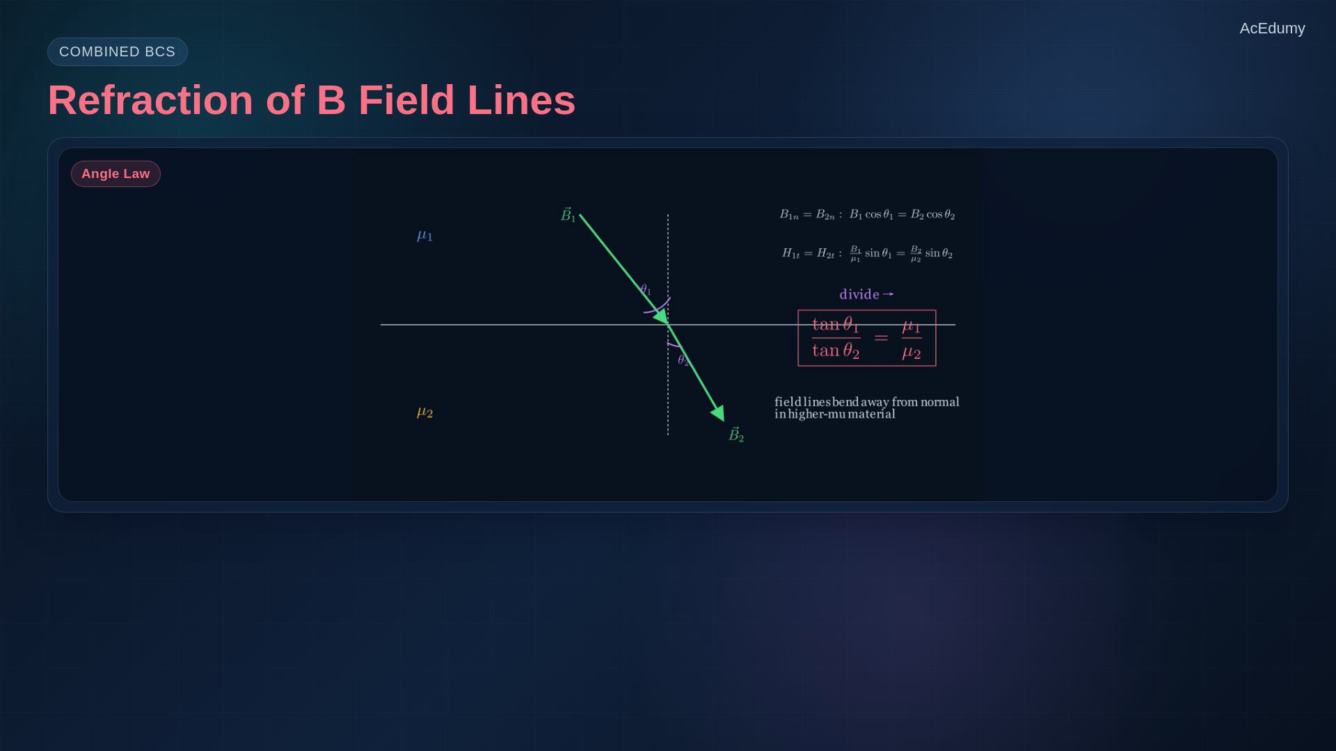
   Here's a quick payoff.

   Combine the two boundary conditions and you get the refraction law for magnetic field lines.

   A B vector in material one hits the interface at angle θ₁ from the normal.

   On the other side it continues at angle θ₂.

   Normal-B continuity:

   $\displaystyle B₁ \cos \theta ₁ = B₂ \cos \theta ₂.$

   For K_s=0, tangential-H continuity gives (B₁/μ₁)sin θ₁ = (B₂/μ₂)sin θ₂.

   Divide the second by the first.

   $\displaystyle \tan \theta ₁/\mu ₁ = \tan \theta ₂/\mu ₂.$

   Refraction law:

   $\displaystyle \tan \theta ₁/\tan \theta ₂ = \mu ₁/\mu ₂.$

   This is the exact same form as electric refraction, just with permeabilities instead of permittivities.

   Field lines bend away from the normal when entering a higher-permeability material — that's why iron pulls magnetic flux lines in.

   Narration transcript

   Here's a quick payoff. Combine the two boundary conditions and you get the refraction law for magnetic field lines. A B vector in material one hits the interface at angle theta-one from the normal. On the other side it continues at angle theta-two. Normal B continuous gives us B-one cosine theta-one equals B-two cosine theta-two. Tangential H continuous — remembering H equals B over mu — gives B-one over mu-one times sine theta-one equals B-two over mu-two times sine theta-two. Divide the second by the first. The B magnitudes cancel, and we're left with: tangent of theta-one over mu-one equals tangent of theta-two over mu-two. Rearrange: tan theta-one over tan theta-two equals mu-one over mu-two. This is the exact same form as electric refraction, just with permeabilities instead of permittivities. Field lines bend away from the normal when entering a higher-permeability material — that's why iron pulls magnetic flux lines in.

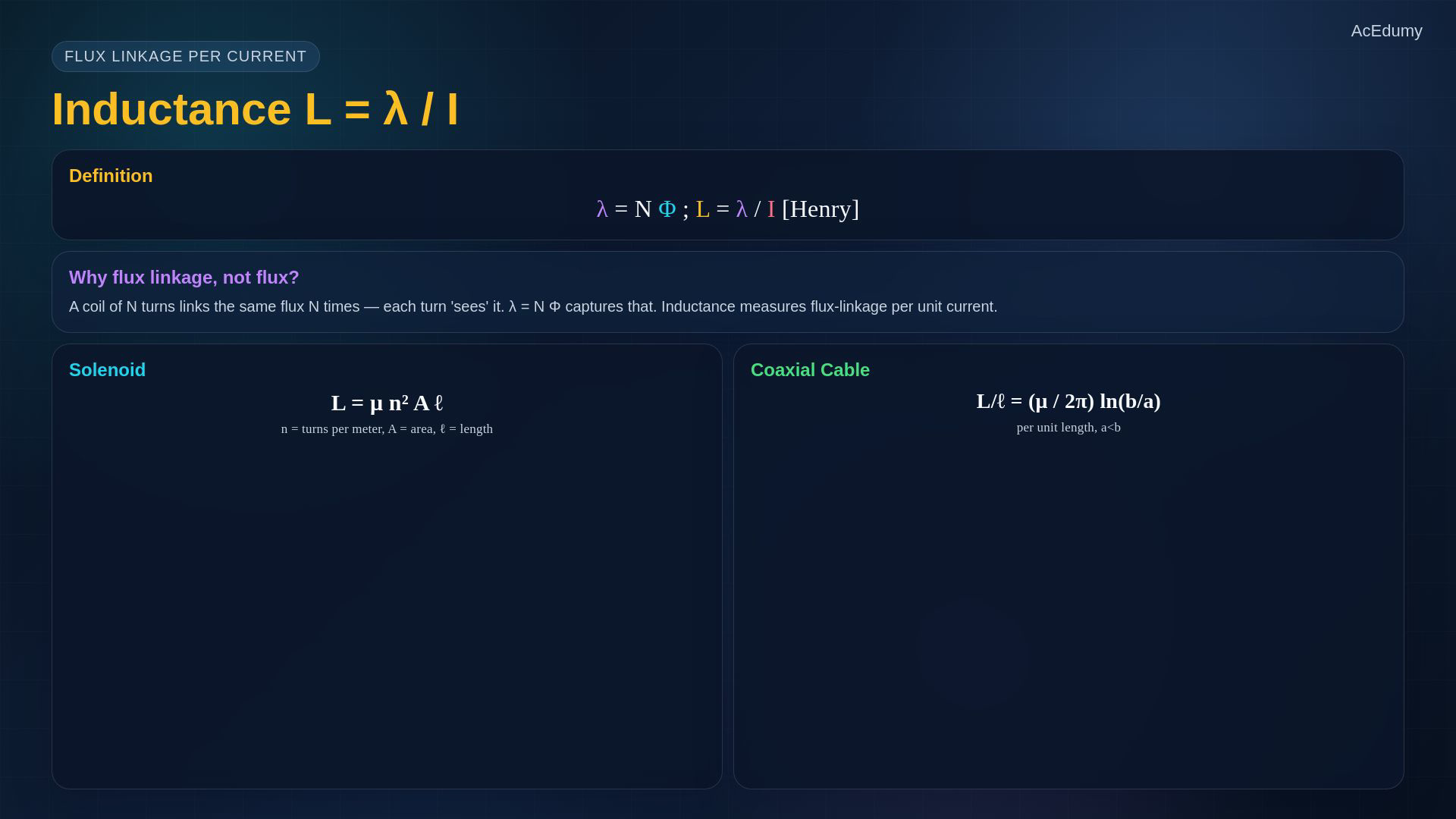
4. 4. Build inductance from flux linkage

   

   Now inductance.

   Take a coil of N turns, carrying current I, and let Φ be the flux through each turn.

   Total flux linkage:

   $\displaystyle \lambda = NΦ.$

   Why flux linkage, not just flux?

   Because if the coil has ten turns, the same flux is linked ten times — each turn 'sees' it.

   For a linear system, inductance is L = λ/I.

   It tells us how much flux linkage a coil can build per unit current.

   The unit is the Henry.

   Let's compute it for a solenoid.

   Inside a long solenoid, H = nI and B = μnI.

   Flux per turn: Φ = BA = μnIA.

   Total linkage: λ = NΦ = NμnIA.

   Since N = nℓ, λ = μn²IAℓ.

   Solenoid inductance:

   $\displaystyle L = \mu n²Aℓ.$

   For a coaxial cable, L′ = (μ/2π)ln(b/a).

   These are the two formulas you'll reach for most often.

   Narration transcript

   Now inductance. Take a coil of N turns, carrying current I, and let Phi be the flux through each turn. The total flux linkage is lambda equals N Phi. Why flux linkage, not just flux? Because if the coil has ten turns, the same flux is linked ten times — each turn 'sees' it. The inductance L is defined as L equals lambda over I. It tells us how much flux linkage a coil can build per unit current. The unit is the Henry. Let's compute it for a solenoid. Inside, H equals n I, so B equals mu n I. Flux per turn is Phi equals B A equals mu n I A. Total flux linkage is lambda equals N Phi equals N mu n I A. But N equals n times ell, the solenoid length, so lambda equals mu n squared I A ell. Divide by I to get L equals mu n squared A ell. For a coaxial cable, a similar derivation gives inductance per unit length equal to mu over two pi times the natural log of b over a, where a is the inner radius and b the outer. These are the two formulas you'll reach for most often.

5. 5. Derive magnetic energy and energy density

   

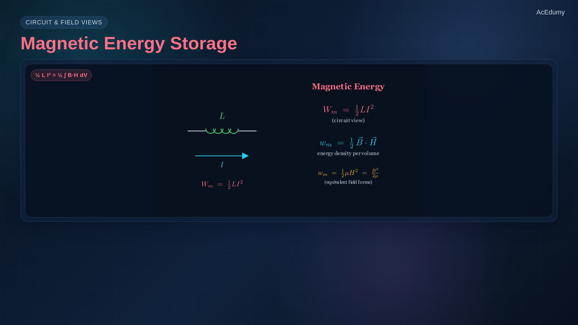
   Finally, energy.

   When you ramp current from zero to I through an inductor, the source has to do work against the back-EMF.

   That work is stored in the magnetic field.

   For constant L, W_m = ∫₀ᴵ Li di = ½LI².

   That's the magnetic energy stored in an inductor — exactly the same structure as one-half C V squared for a capacitor.

   The factor ½ comes from ∫₀ᴵ i di, not from assuming a linear rise in time.

   The result holds for any current ramp waveform as long as L is constant.

   We can also express this field by field.

   In a linear medium, w_m = ½B·H = ½μH² = B²/(2μ).

   Integrating over volume gives ∫w_m dv = ½LI².

   Two views of the same energy: circuit-based with L and I, and field-based with B and H.

   Both are essential — circuit engineers use the first, field theorists the second.

   Narration transcript

   Finally, energy. When you ramp current from zero to I through an inductor, the source has to do work against the back-EMF. That work is stored in the magnetic field. Integrate voltage times current over time: the integral of L d I by d t times I, from zero to I, gives one-half L I squared. That's the magnetic energy stored in an inductor — exactly the same structure as one-half C V squared for a capacitor. Why the one-half? Because the current rises linearly, so average current times final current gives half the product. We can also express this field by field. The energy density at each point of space is one-half B dotted with H, or equivalently one-half mu H squared, or B squared over two mu. Integrate this over all space and you recover the total one-half L I squared. Two views of the same energy: circuit-based with L and I, and field-based with B and H. Both are essential — circuit engineers use the first, field theorists the second.

6. 6. Close the static electromagnetics block

   

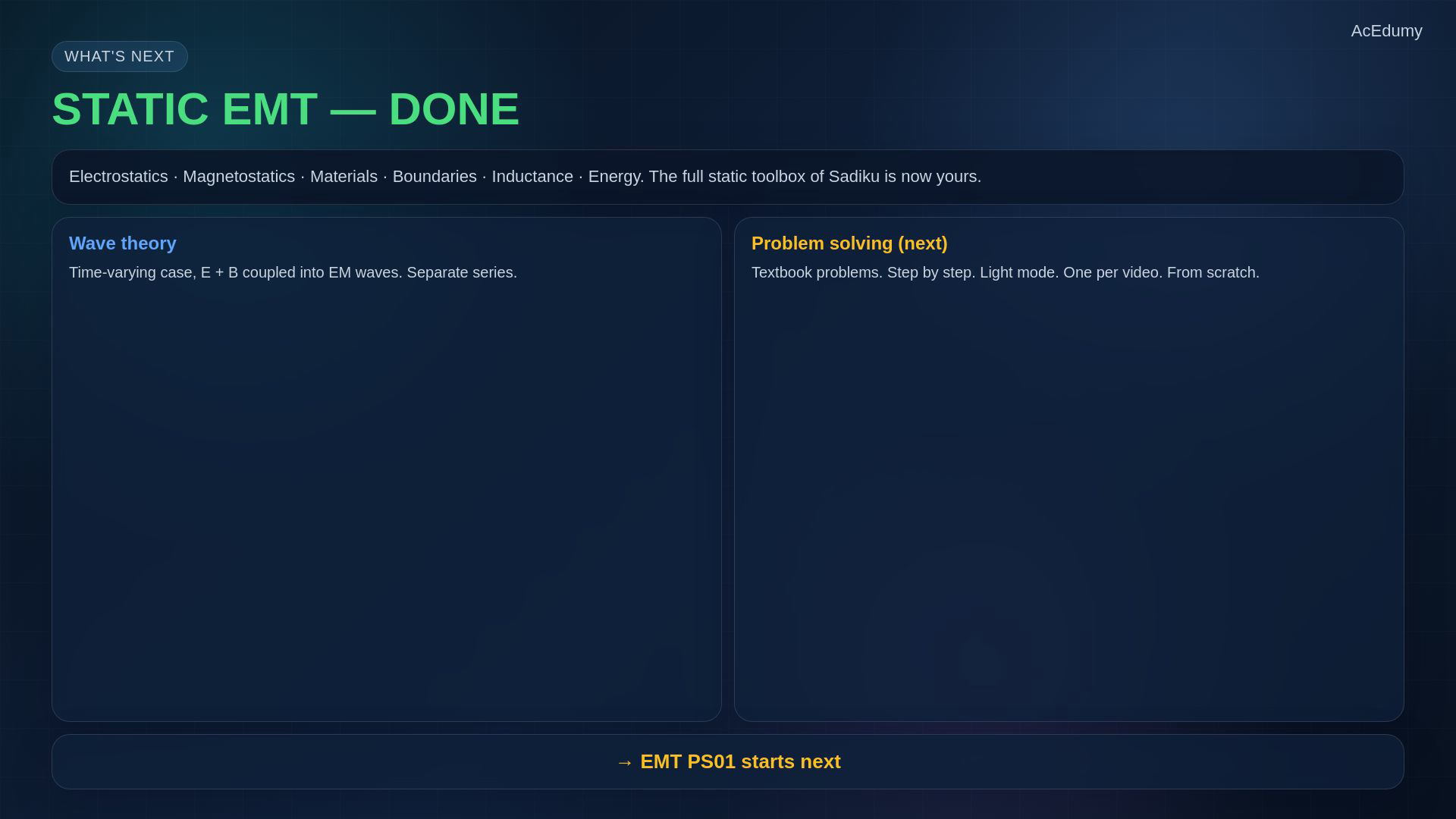
   And that closes the static block.

   Over the last many videos we built up electrostatics from Coulomb to Gauss to potential to Laplace, magnetostatics from Biot-Savart to Ampère to the flux density B, and we covered materials, forces, boundaries, inductance, and magnetic energy.

   Every static chapter of Sadiku is now in your toolbox.

   The course turns next.

   Wave theory — the time-varying case, where E and B couple into electromagnetic waves — is a separate series.

   For the next several videos, we switch to problem solving: textbook exercises, one per video, step by step, everything explained from scratch.

   The theory is built; now we use it.

   Narration transcript

   And that closes the static block. Over the last many videos we built up electrostatics from Coulomb to Gauss to potential to Laplace, magnetostatics from Biot-Savart to Ampère to the flux density B, and we covered materials, forces, boundaries, inductance, and magnetic energy. Every static chapter of Sadiku is now in your toolbox. The course turns next. Wave theory — the time-varying case, where E and B couple into electromagnetic waves — is a separate series. For the next several videos, we switch to problem solving: textbook exercises, one per video, step by step, everything explained from scratch. The theory is built; now we use it.

Source video: Electromagnetic Theory (v2) #23 | Boundary Conditions, Inductance & Magnetic Energy (7:01)