Electromagnetic Theory · Poisson's and Laplace's Equations
#15 Deriving Poisson's and Laplace's equations from Gauss's law, the Laplacian in three coordinate systems, a boundary-value workflow, and an electrohydrodynamic pump example
Derive Poisson and Laplace equations, solve potential from boundary conditions, and calculate the pressure of an EHD pump.
Question
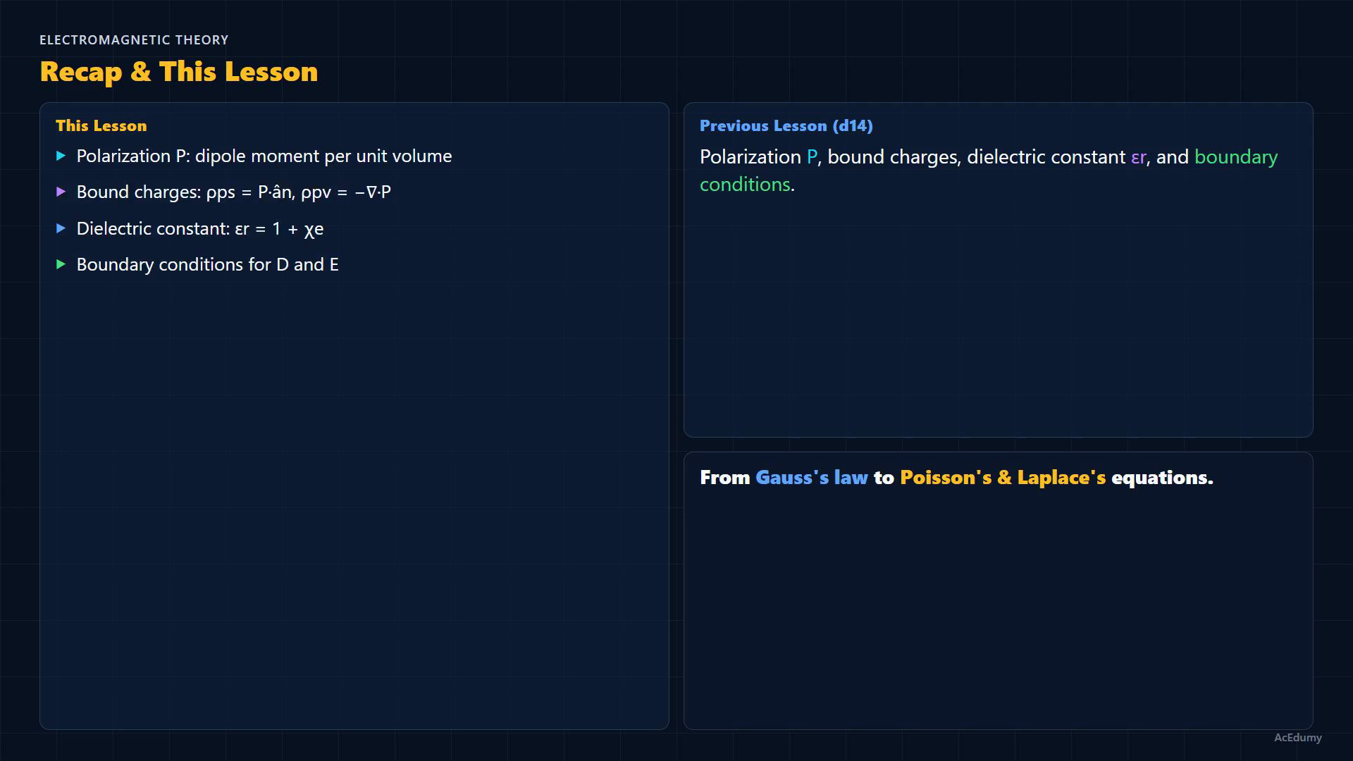
Derive Poisson's and Laplace's equations from Gauss's law; write the Laplacian in Cartesian, cylindrical, and spherical coordinates, apply the boundary-value workflow, and calculate the EHD pump pressure.
Written solution and narration transcript(shows the full solution)
Below are all the lines written in the notebook together with the full narration transcript.
1. Move from dielectrics to potential equations
Poisson's equation applies where charge is present; Laplace's equation applies in charge-free regions, with boundary conditions fixing the solution. In our last lesson, we explored polarization and dielectrics.We defined the polarization vector P, derived bound charge densities, and introduced the dielectric constant εr and permittivity ε.We also established boundary conditions for D and E at dielectric interfaces.Today, we move to one of the most powerful tools in electrostatics: Poisson's and Laplace's equations.These equations let us find the electric potential V when we know only the boundary conditions, not the charge distribution everywhere.Narration transcript
In our last lesson, we explored polarization and dielectrics. We defined the polarization vector P, derived bound charge densities, and introduced the dielectric constant epsilon r and permittivity epsilon. We also established boundary conditions for D and E at dielectric interfaces. Today, we move to one of the most powerful tools in electrostatics: Poisson's and Laplace's equations. These equations let us find the electric potential V when we know only the boundary conditions, not the charge distribution everywhere.
2. Derive Poisson's and Laplace's equations
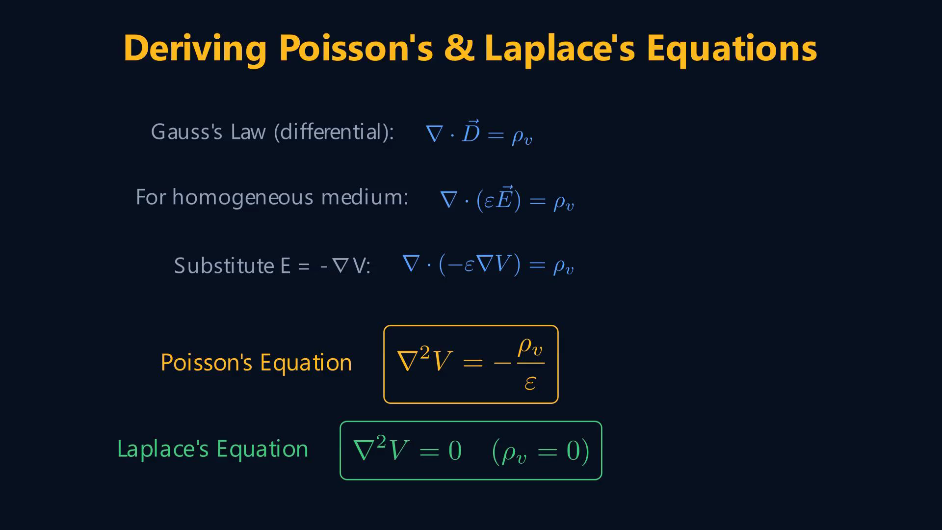
Poisson's equation applies where charge is present; Laplace's equation applies in charge-free regions, with boundary conditions fixing the solution. Let's derive these equations from what we already know.Start with Gauss's law:For a linear, isotropic, homogeneous medium D = εE, so ∇·(εE) = ρv.We also know E = −∇V.Substitution gives ∇·(−ε∇V) = ρv.If ε is constant throughout the region, we can pull it out: negative ε times the ∇²V equals ρv.Poisson's equation:When there is no free charge in the region, ρv equals zero, and Poisson's equation simplifies to Laplace's equation: ∇²V equals zero.Narration transcript
Let's derive these equations from what we already know. We start with Gauss's law in differential form: divergence of D equals the volume charge density rho v. For a linear, isotropic, homogeneous medium, D equals epsilon E, so divergence of epsilon E equals rho v. We also know that E equals negative gradient of V. Substituting this into Gauss's law, we get: divergence of negative epsilon gradient V equals rho v. If epsilon is constant throughout the region, we can pull it out: negative epsilon times the Laplacian of V equals rho v. This gives us Poisson's equation: Laplacian of V equals negative rho v over epsilon. When there is no free charge in the region, rho v equals zero, and Poisson's equation simplifies to Laplace's equation: Laplacian of V equals zero.
3. Write the Laplacian in three coordinate systems
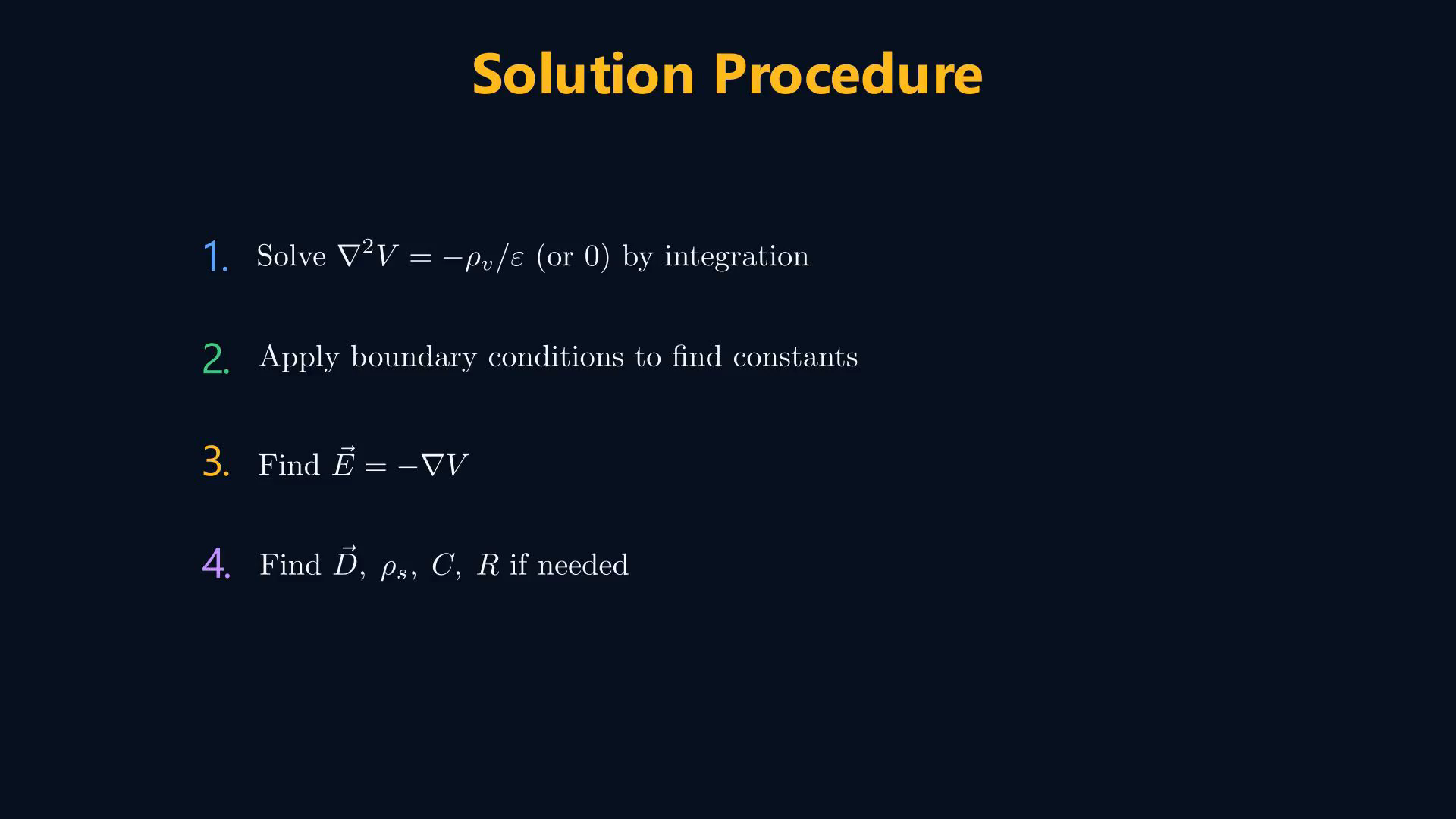
Poisson's equation applies where charge is present; Laplace's equation applies in charge-free regions, with boundary conditions fixing the solution. The ∇²V takes different forms in each coordinate system.In Cartesian coordinates, it is the sum of the second partial derivatives with respect to x, y, and z.In cylindrical coordinates, the Laplacian has a one over rho term with a rho derivative, a one over rho squared term with the phi derivative, and a z derivative.In spherical coordinates, it has a one over r squared term with an r derivative, a one over r squared sine theta term with the theta derivative, and a one over r squared sine squared theta term with the phi derivative.The general procedure to solve a boundary-value problem is: Step one, solve Laplace's or Poisson's equation by direct integration to get V with unknown constants.Step two, apply boundary conditions to determine those constants.Step three: find E from E = −∇V.Step four, if needed, find D, surface charge, or capacitance.Narration transcript
The Laplacian of V takes different forms in each coordinate system. In Cartesian coordinates, it is the sum of the second partial derivatives with respect to x, y, and z. In cylindrical coordinates, the Laplacian has a one over rho term with a rho derivative, a one over rho squared term with the phi derivative, and a z derivative. In spherical coordinates, it has a one over r squared term with an r derivative, a one over r squared sine theta term with the theta derivative, and a one over r squared sine squared theta term with the phi derivative. The general procedure to solve a boundary-value problem is: Step one, solve Laplace's or Poisson's equation by direct integration to get V with unknown constants. Step two, apply boundary conditions to determine those constants. Step three, find E from E equals negative gradient of V. Step four, if needed, find D, surface charge, or capacitance.
4. Solve the EHD pump example
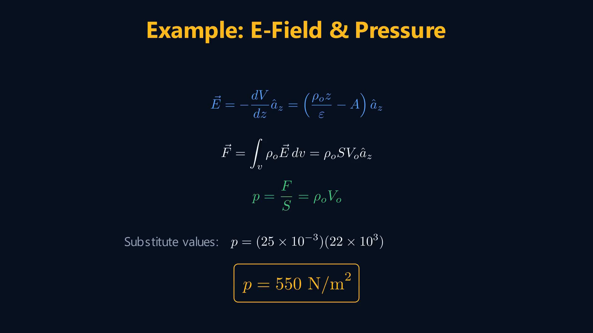
Poisson's equation applies where charge is present; Laplace's equation applies in charge-free regions, with boundary conditions fixing the solution. Let's work through Example 6.1 from Sadiku.An electrohydrodynamic pump has two parallel electrodes separated by distance d.The region between them contains a uniform charge density ρ₀.The left electrode is at voltage V₀, and the right electrode at zero volts.Find the pressure of the pump.Given ρ₀ = 25 mC/m³.The left electrode is at V₀ = 22 kV.Step one: Since ρv is not zero, we use Poisson's equation.The potential depends only on z, so the Laplacian reduces to d² V over d z² equals negative ρ₀ over ε.Step two: Integrate once.d V over d z equals negative ρ₀ z over ε, plus a constant A.Step three: Integrate again.V equals negative ρ₀ z² over 2 ε, plus A z, plus B.Step four: Apply boundary conditions.V(0) = V₀, so B = V₀.Thus B = 22,000 V.V(d) = 0 ⇒ 0 = −ρ₀d²/(2ε) + Ad + V₀.Step five: E = −dV/dz.The net force is F = ∫ρ₀E dv.The integral gives F = ρ₀SV₀az.Pressure is p = F/S = ρ₀V₀.p = 25×10⁻³×22×10³ Pa.The result is p = 550 N/m² = 550 Pa.Narration transcript
Let's work through Example 6.1 from Sadiku. An electrohydrodynamic pump has two parallel electrodes separated by distance d. The region between them contains a uniform charge density rho o. The left electrode is at voltage V o, and the right electrode at zero volts. Find the pressure of the pump. Given values: rho o equals 25 milliCoulombs per cubic metre. V o equals 22 kilovolts. Step one: Since rho v is not zero, we use Poisson's equation. The potential depends only on z, so the Laplacian reduces to d squared V over d z squared equals negative rho o over epsilon. Step two: Integrate once. d V over d z equals negative rho o z over epsilon, plus a constant A. Step three: Integrate again. V equals negative rho o z squared over 2 epsilon, plus A z, plus B. Step four: Apply boundary conditions. At z equals 0, V equals V o, so B equals V o. That gives us B equals 22000 volts. At z equals d, V equals 0, so zero equals negative rho o d squared over 2 epsilon, plus A d, plus V o. Solving for A: A equals rho o d over 2 epsilon, minus V o over d. Step five: The electric field is E equals negative d V over d z. This gives E equals rho o z over epsilon minus A, in the z direction. The net force on the charge is F equals the integral of rho o times E over the volume. After evaluating, the force simplifies to F equals rho o times S times V o, in the z direction. The pressure is force per unit area: p equals rho o times V o. Substituting: p equals 25 times 10 to the negative 3, times 22 times 10 to the 3. This gives p equals 550 Newtons per square metre.
5. Review the Poisson–Laplace workflow
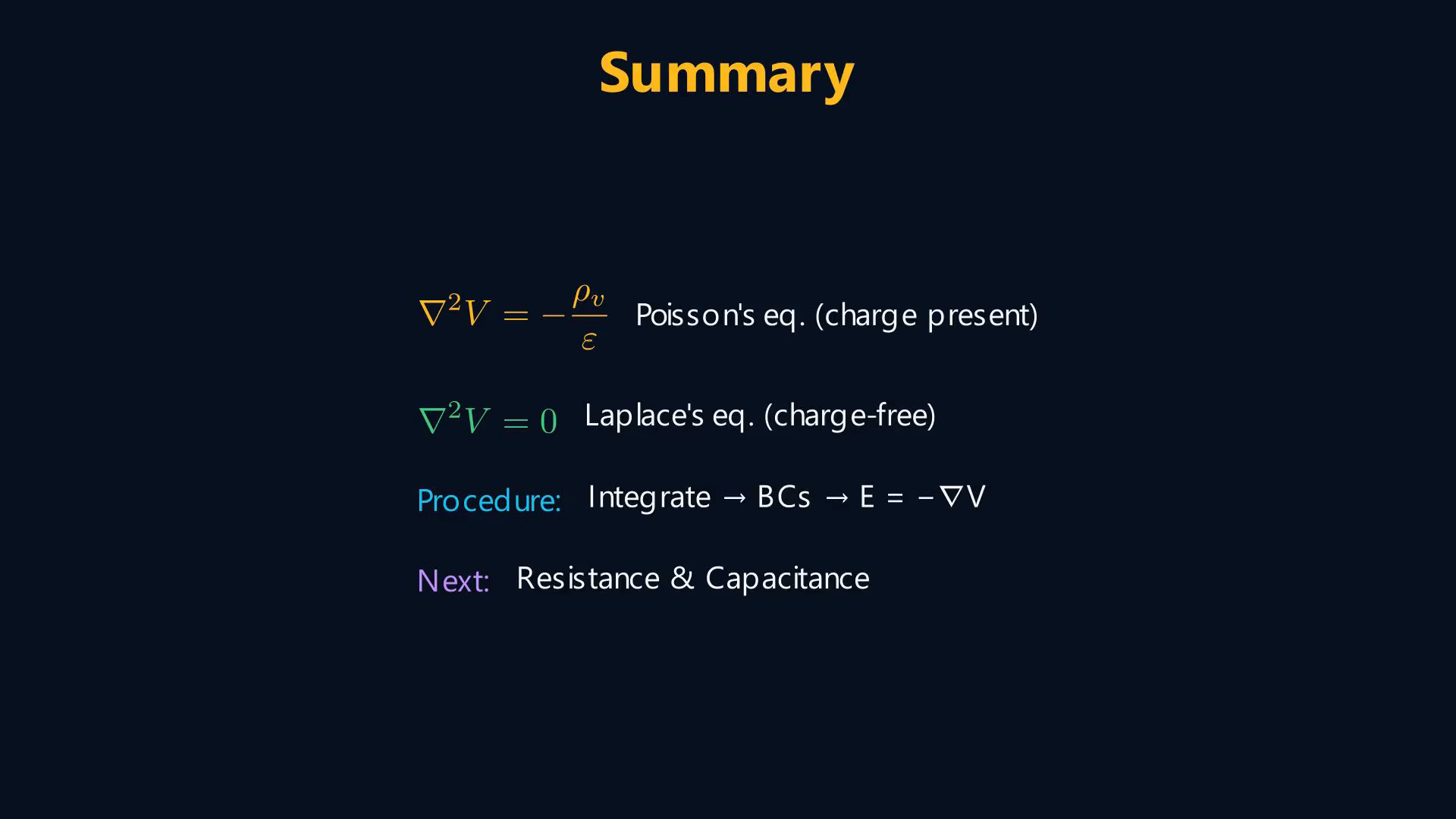
Poisson's equation applies where charge is present; Laplace's equation applies in charge-free regions, with boundary conditions fixing the solution. Let's summarize.Poisson's equation, ∇²V equals negative ρv over ε, applies when free charge is present.Laplace's equation ∇²V = 0 applies in charge-free regions.The solution procedure is: integrate the equation, apply boundary conditions, then find E from the gradient of V.In our next lesson, we'll apply these equations to find resistance and capacitance of various geometries.Narration transcript
Let's summarize. Poisson's equation, Laplacian of V equals negative rho v over epsilon, applies when free charge is present. Laplace's equation, Laplacian of V equals zero, applies in charge-free regions. The solution procedure is: integrate the equation, apply boundary conditions, then find E from the gradient of V. In our next lesson, we'll apply these equations to find resistance and capacitance of various geometries.
Source video: Electromagnetic Theory (v2) #15 Poisson's & Laplace's Equations (5:49)