Circuit Theory 2 · Poles, zeros, initial value and final value

#16 Reduced rational transforms, causal modes, and conditions for the two endpoint theorems

Read poles and zeros, then verify initial and final values with explicit theorem conditions and readable fractions.

Question

Reviewed reference card from the existing English final, showing transform behavior or an endpoint calculation. — Original-video reference. Three clipped or overlapping graphics use other cards from this same final; complete formulas and conditions appear in the notebook lines.

Read F(s)=(2s+5)/((s+1)(s+3)) before inversion: find its poles −1 and −3, zero −2.5, finite initial value 2 and final value 0. Independently check Y(s)=10/(s(s+2)): initial 0 and final 5. Signals are ordinary causal functions with finite right-hand initial limits, not distributions; no impulse or impulse derivative is present at the origin. Positive-time modal formulas extend causally with u(t). Let s=σ+jω_s, with σ the real part; the first ROC is σ>−1 and the step-response ROC is σ>0. Cancel common factors before identifying poles and finite zeros. Include the numerator gain; zero locations alone do not specify weights. Exact output cancellation is not proof that internal modes vanish or that a circuit is internally stable. F is a signal transform, not automatically a circuit transfer function. A simple pole gives an exponential; a pole of order m permits time powers zero through m−1. The displayed repeated example is a double pole. For a real-coefficient pair −α±jω with real ω>0, damping requires α>0; α=0 gives sustained oscillation and α<0 gives growth. The source's unqualified damped-oscillation sentence is retained unchanged in say and MP3 and remains a manual teaching-QA caveat, not a corrected source recording. The initial theorem takes s to +∞ along the positive real axis, not along the imaginary axis. For the rational final-value test here every pole of reduced sF must be strictly in the open left half-plane, including no remaining pole at the origin. The symbols f_∞ and y_∞ denote time limits as t tends to +∞. Arrows in displayed limits mean approach at the destination stated in the sentence, not equality for all s or t. Decay rates have inverse-time units; no unspecified voltage or current units are invented. Recombine the step response as 5/s−5/(s+2) to obtain 5(1−exp(−2t))u(t). All nine original final frames were inspected. The pole map's σ label is covered, the modal fast/slow labels overlap ticks, and the step-response curve's origin is outside the final frame. Those three roles reuse readable reference cards from the same final; no corrected video or animation was generated. The notebook displays full formatted equations and assumptions. Remaining old raster typography, unqualified source narration, and source card/narration differences remain manual teaching QA. This is an unpublished draft, not full human listening, full motion QA or publication approval.

Written solution and narration transcript(shows the full solution)

Below are all the lines written in the notebook together with the full narration transcript.

1. Read behavior before full inversion
Original-video reference. Three clipped or overlapping graphics use other cards from this same final; complete formulas and conditions appear in the notebook lines.
Previous lesson: decompose a rational transform, then invert each term.
Now first ask what its algebra already reveals.
Can we find modes and endpoints before computing the full inverse?
Yes: roots and two conditional limit checks provide useful information.
After cancelling common factors, poles determine modes of this causal signal; natural circuit modes also require a circuit model.
The numerator, including its gain, sets modal weights and may cancel denominator factors.
Initial and final values are endpoint checks, each with its own conditions; neither determines the full waveform.
Narration transcript
In the previous lesson, we decomposed F of s and then inverted each piece. Now we ask a faster question. Before doing the full inverse Laplace, what can we already read from the expression? A lot. The denominator roots, called poles, tell us which natural time modes can appear. The numerator roots, called zeros, tell us how those modes are shaped, weighted, or sometimes cancelled. And two limit theorems let us check the beginning and the end of the waveform without expanding the whole answer.
2. Find roots after cancellation
Original-video reference. Three clipped or overlapping graphics use other cards from this same final; complete formulas and conditions appear in the notebook lines.
Cancel common factors before identifying finite poles and zeros:
$\displaystyle F\left(s\right)=\frac{N\left(s\right)}{D\left(s\right)}$
For a nonzero reduced rational function, finite zeros are numerator roots:
$\displaystyle N\left(z\right)=0$
Uncancelled denominator roots are poles:
$\displaystyle D\left(p\right)=0$
The causal example has ROC σ>−1 and poles −1 and −3:
$\displaystyle F\left(s\right)=\frac{2 s+5}{\left(s+1\right)\left(s+3\right)}$
Solve the numerator equation; there is no common factor:
$\displaystyle 2 z+5=0, z=-\frac{5}{2}=-2.5$
In an s-plane diagram, crosses denote poles:
$\displaystyle p_{1}=-1, p_{2}=-3$
An open circle denotes the zero; the horizontal coordinate is the real part σ.
The two causal exponentials and their weights, for positive time:
$\displaystyle f\left(t\right)=\left(\frac{3}{2}\right)e^{-t}+\left(\frac{1}{2}\right)e^{-3 t}$
Narration transcript
Start with a rational transform, F of s equals N of s over D of s. Zeros are the roots of the numerator. Poles are the roots of the denominator. For the example from last lesson, two s plus five over s plus one times s plus three, the poles are at minus one and minus three. The zero is at minus two point five. On the s-plane, poles are the X marks. The zero is the open circle. The poles create the allowed exponential modes; the zero changes the mixture.
3. Connect poles to causal time modes
Original-video reference. Three clipped or overlapping graphics use other cards from this same final; complete formulas and conditions appear in the notebook lines.
Read the pole location, multiplicity and the causal assumption together.
For a simple real pole, with a positive in the decaying case and positive time:
$\displaystyle p=-a, g\left(t\right)=A e^{-a t}$
For a double pole, include the constant and time terms; higher orders add higher powers:
$\displaystyle g\left(t\right)=\left(A+B t\right)e^{-a t}$
For a real-coefficient conjugate pair −α±jω with ω>0, damping requires α>0:
$\displaystyle g\left(t\right)=e^{-\alpha t}\left[A \cos \left(\omega t\right)+B \sin \left(\omega t\right)\right]$
A complex pair is not automatically damped: zero real part gives sustained oscillation, positive real part gives growth.
A pole of order m permits time powers from zero through m−1; individual coefficients may vanish.
Compare decaying real modes for positive time:
$\displaystyle a_{\mathrm{fast}}=4, a_{\mathrm{slow}}=1, e^{-4 t}<e^{-t}$
Among left-half-plane poles, a real part closer to zero gives slower envelope decay.
An uncancelled right-half-plane pole gives a growing causal mode; output cancellation alone cannot prove internal stability.
Narration transcript
Here is the key reading rule. A pole at minus a creates an e to the minus a t mode. If the pole is repeated, the same decay comes with a t multiplier. A complex conjugate pole pair gives a damped oscillation. So poles do more than mark denominator roots. They tell you the building blocks of the time response. Farther left means faster decay. Closer to the imaginary axis means slower decay. Right half-plane poles mean growth, which is a warning sign.
4. Understand numerator weights and cancellation
Original-video reference. Three clipped or overlapping graphics use other cards from this same final; complete formulas and conditions appear in the notebook lines.
Zeros play a different role from poles.
A zero does not itself add an exponential mode to the strictly proper rational signal.
In this example, the numerator fixes both modal weights:
$\displaystyle F\left(s\right)=\frac{\frac{3}{2}}{s+1}+\frac{\frac{1}{2}}{s+3}$
An exact common factor may cancel in the output expression; that does not prove the internal circuit mode is absent or stable.
Two responses can have the same poles but different numerators and gain.
Keep gain as well as zero locations: zeros alone do not specify all the modal weights.
Narration transcript
Zeros behave differently. A zero usually does not create a new time mode. Instead, it shapes how the pole modes combine. It can make one mode stronger, weaken another, flip a sign, or create an exact cancellation if it lands on a pole. That is why two circuits can have the same poles, but different-looking responses. The poles give the possible modes; the zeros help decide how those modes are mixed at the output.
5. Check the finite initial value
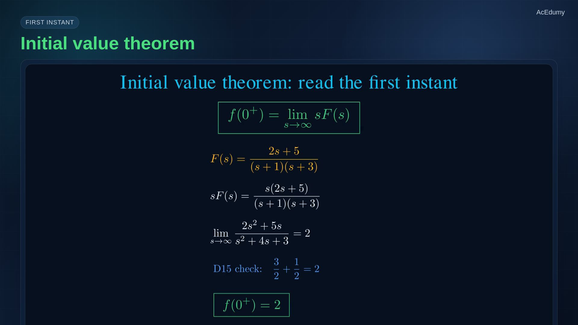
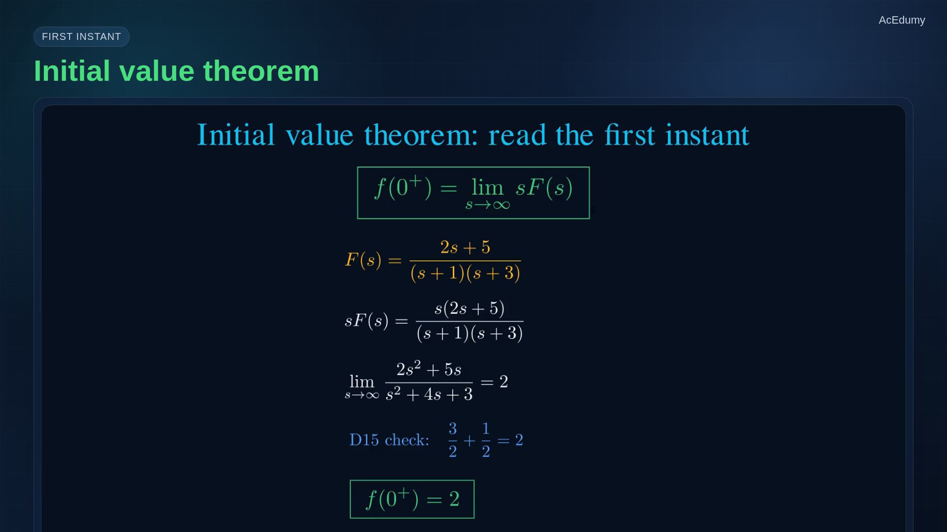
Original-video reference. Three clipped or overlapping graphics use other cards from this same final; complete formulas and conditions appear in the notebook lines.
The initial value is a finite right-hand time limit; exclude impulses and their derivatives at the origin.
For these ordinary causal signals, f at zero plus is the limit of sF(s) as positive real s tends to positive infinity.
Increasing positive real s suppresses later time more strongly in the Laplace integral; this is not a sweep along the imaginary axis.
Multiply the complete transform by s:
$\displaystyle s F\left(s\right)=\frac{s\left(2 s+5\right)}{\left(s+1\right)\left(s+3\right)}$
Divide numerator and denominator by s squared, then take s to positive infinity:
$\displaystyle s F\left(s\right)=\frac{2+\frac{5}{s}}{1+\frac{4}{s}+\frac{3}{s^{2}}}\to 2$
Check the right-hand time limit independently:
$\displaystyle f\left(0^{+}\right)=\left(\frac{3}{2}\right)+\left(\frac{1}{2}\right)=2$
Narration transcript
The initial value theorem reads the very beginning of the waveform. If F of s is the transform of f of t, then f of zero plus equals the limit, as s goes to infinity, of s times F of s. Intuitively, large s emphasizes the earliest instant. For our example, multiply F of s by s. At very large s, the leading terms dominate: s times two s plus five over s plus one times s plus three tends to two. That matches the time-domain answer from last lesson: three over two plus one over two equals two.
6. Apply the final-value stability gate
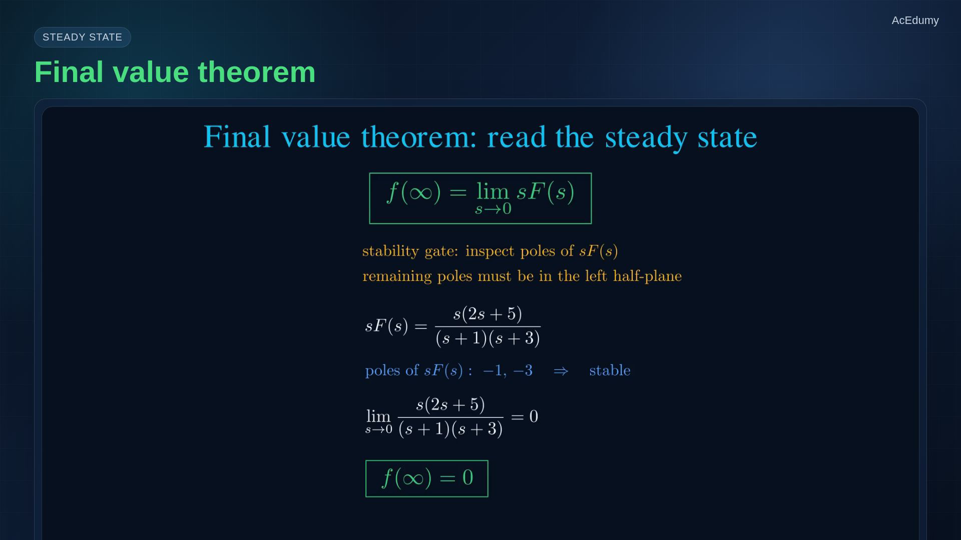
Original-video reference. Three clipped or overlapping graphics use other cards from this same final; complete formulas and conditions appear in the notebook lines.
Before using the final-value theorem, check every pole of the reduced product sF.
After the pole check, the final time limit is the limit of sF(s) as positive real s approaches zero; f_∞ denotes that time limit.
For the rational signals here, all remaining poles of sF must lie strictly in the open left half-plane.
Any remaining pole at the origin, elsewhere on the imaginary axis, or in the right half-plane fails this gate.
The remaining poles are −1 and −3; after the gate passes:
$\displaystyle f_{\infty }=\frac{0\left(2\cdot 0+5\right)}{\left(0+1\right)\left(0+3\right)}=0$
An independent check as positive time tends to infinity:
$\displaystyle f\left(t\right)=\left(\frac{3}{2}\right)e^{-t}+\left(\frac{1}{2}\right)e^{-3 t}\to 0$
Narration transcript
The final value theorem reads the steady state, but only after a stability check. The formula is f at infinity equals the limit, as s goes to zero, of s times F of s. But this is valid only if all remaining poles of s F of s are in the left half-plane. If there is a right half-plane pole, or a sustained imaginary-axis oscillation, the theorem can lie to you. In the same example, s F of s goes to zero at s equals zero, so the final value is zero. Both exponential modes decay, so the answer makes sense.
7. Verify both endpoints of a step response
Original-video reference. Three clipped or overlapping graphics use other cards from this same final; complete formulas and conditions appear in the notebook lines.
Now check an independent causal step-response example.
The whole denominator is a product; the causal ROC is σ>0:
$\displaystyle Y\left(s\right)=\frac{10}{s\left(s+2\right)}$
First multiply the entire transform by s:
$\displaystyle s Y\left(s\right)=\frac{10 s}{s\left(s+2\right)}$
Cancel the common factor; the remaining pole is −2:
$\displaystyle s Y\left(s\right)=\frac{10}{s+2}$
Take s to positive infinity along the real axis:
$\displaystyle s Y\left(s\right)=\frac{10}{s+2}\to 0$
The finite right-hand initial value is therefore:
$\displaystyle y\left(0^{+}\right)=0$
Before taking s to zero, confirm that the only remaining pole −2 lies strictly in the left half-plane.
After that check, the final value follows:
$\displaystyle y_{\infty }=\frac{10}{0+2}=5$
The endpoints agree with the causal inverse, including the unit step:
$\displaystyle y\left(t\right)=5\left(1-e^{-2 t}\right) u\left(t\right)$
Narration transcript
Now use the theorems on a step response. Let Y of s equal ten over s times s plus two. First multiply by s. Then s Y of s is ten over s plus two. For the initial value, let s go to infinity. Ten over s plus two goes to zero, so y of zero plus is zero. For the final value, let s go to zero. Ten over two is five, so the output settles at five. Without doing the full inverse Laplace, we know the curve starts at zero and ends at five.
8. Avoid value-theorem traps
Original-video reference. Three clipped or overlapping graphics use other cards from this same final; complete formulas and conditions appear in the notebook lines.
Three traps: the wrong pole set, missing convergence conditions, and confusing poles with zeros.
A simple pole at the origin in Y may cancel when forming sY; it is not by itself a final-value failure.
Test the reduced product, not the original denominator:
$\displaystyle s Y\left(s\right)=\frac{10}{s+2}, p=-2$
A remaining right-half-plane pole invalidates this final-value test; remaining imaginary-axis poles also fail it.
Do not assign a new exponential mode to a numerator zero.
The numerator and gain determine modal weights and possible output cancellations.
Poles describe signal modes here; claims about natural circuit modes and internal stability need the actual circuit model.
Narration transcript
Three traps matter. First, a pole at the origin in Y of s is not automatically a final value problem. The test is on the poles of s times Y of s, after the multiplication. Second, if any remaining pole is in the right half-plane, the final value theorem is invalid. Third, do not treat a zero as if it creates its own exponential mode. Zeros shape the mixture. Poles create the natural modes.
9. Keep modes and endpoint conditions together
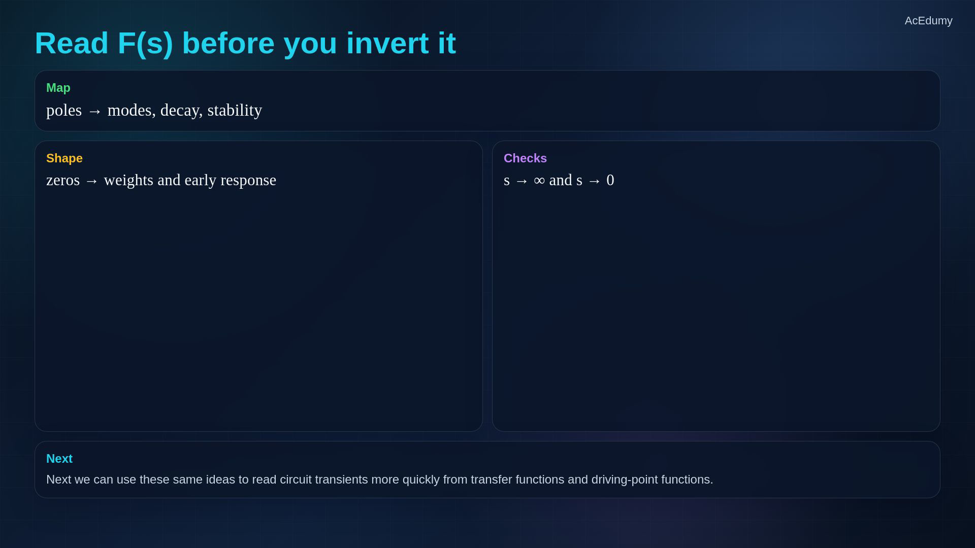
Original-video reference. Three clipped or overlapping graphics use other cards from this same final; complete formulas and conditions appear in the notebook lines.
Summary: roots describe modes; conditional limits check endpoints.
Reduce the rational expression before identifying poles and their multiplicities.
Numerator roots and gain shape the mixture, including possible cancellations.
For a finite ordinary right-hand value with no origin impulse, the initial theorem uses positive real s approaching infinity.
For the final theorem, every remaining pole of the reduced product sF must lie strictly in the open left half-plane.
Next: s-domain models of resistors, inductors and capacitors with their initial conditions.
Narration transcript
Summary. Poles are denominator roots, and they reveal the natural time modes. Zeros are numerator roots, and they shape the mixture of those modes. The initial value theorem reads the first instant from the high-s limit. The final value theorem reads the steady state from the low-s limit, but only after the stability gate is passed. Next, we turn resistors, inductors, and capacitors into s-domain models with initial conditions.