Circuit Theory 1 · First-Order Transients
#45 Transient Analysis #45 — RC pulse-input response
Decomposes a finite pulse into two steps and solves RC charging before T, discharge afterward, and a numerical example.
Question
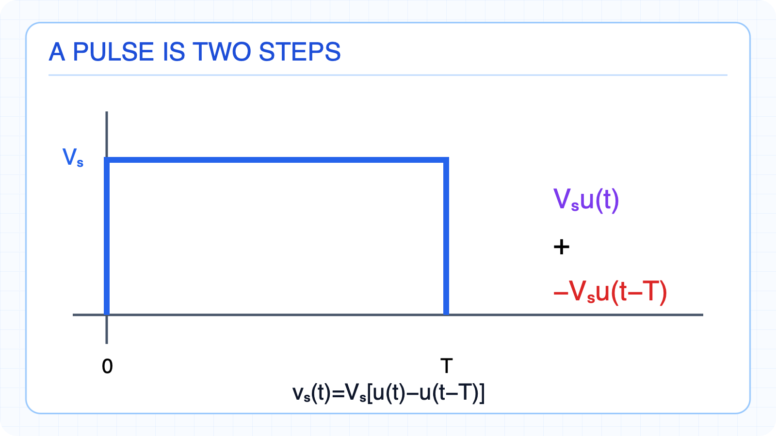
A 5 V pulse is applied to an uncharged RC circuit with R=10 kΩ and C=100 μF for 0≤t<2 s. Find piecewise v_C(t), v_C(2), v_C(3), and v_C(5).
Written solution and narration transcript(shows the full solution)
Below are all the lines written in the notebook together with the full narration transcript.
1. A pulse is the sum of two steps
The positive step at zero is canceled by a delayed negative step at T. The source is on only for 0≤t<TApply a +VS step at t=0Apply a −VS step at t=TThe second step cancels the firstPulse = positive step + delayed negative stepSolve each step response separatelyUse local time t−T for the delayed responseAdd the results by superpositionNarration transcript
What happens when a voltage source is applied for only a limited time? This is called a pulse input. We can express a pulse mathematically as: v s of t equals V S times u of t minus u of t minus T. In other words, the source turns on at t equals zero, and turns off at t equals T. The key idea is superposition: we treat the pulse as the sum of two step inputs. The first step turns on at t equals zero with amplitude V S. The second step turns on at t equals T with amplitude negative V S, effectively canceling the first. We solve each step response separately, then add the results.
2. Two regions of the RC pulse response
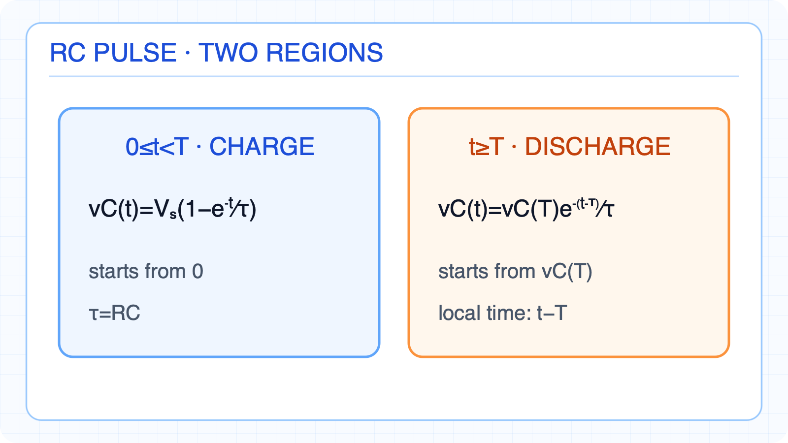
Source-driven charging before T and natural discharge from v_C(T) afterward. The capacitor starts unchargedFor 0≤t<T, the source is connectedτ=RCvC is continuous at t=TThe source turns off after TThe new initial value is vC(T)For t≥T:Charge first, then natural dischargeNarration transcript
Let us derive the RC pulse response using superposition. For the first step at t equals zero, the capacitor charges with: v one of t equals V S times one minus e to the negative t over tau. This is just the standard step response we already know. Now at t equals T, a negative step arrives. The response to this second step is: v two of t equals negative V S times one minus e to the negative t minus T over tau, valid for t greater than or equal to T. Adding both responses, we get two regions. For zero less than t less than T: v c of t equals V S times one minus e to the negative t over tau. The capacitor simply charges. For t greater than or equal to T: v c of t equals V S times e to the negative t minus T over tau minus e to the negative t over tau. This can be rewritten as the voltage at the moment T, times an exponential decay from that point.
3. 5 V, 2 s RC pulse example
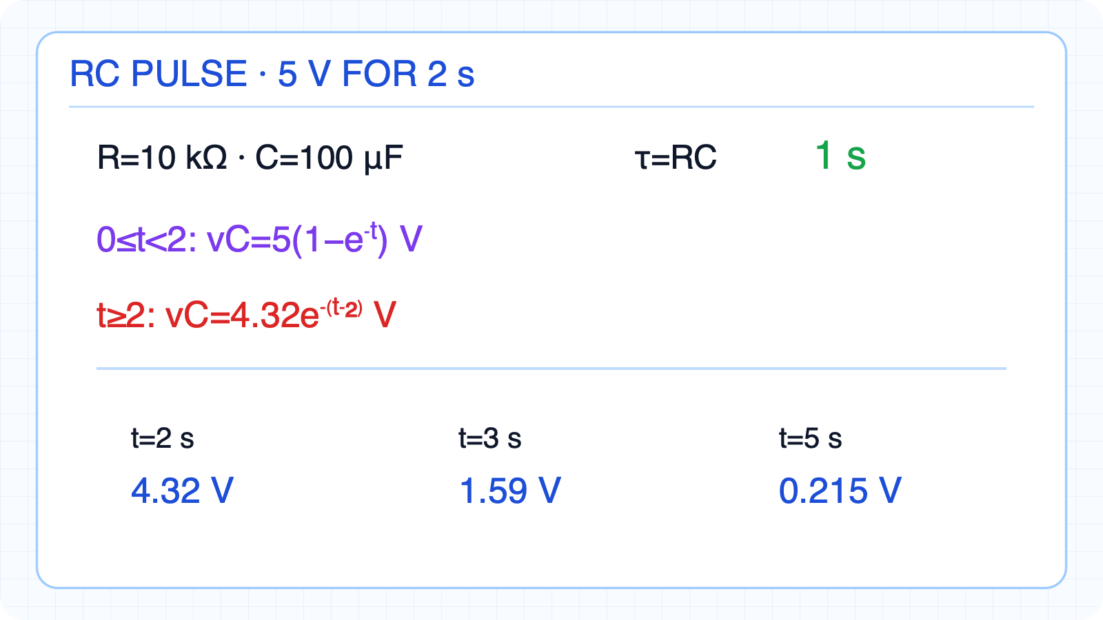
Voltages at 2, 3, and 5 seconds with a one-second time constant. τ=RC=1 s0≤t<2:Voltage at the end of the pulset≥2:Discharge starts from 4.32 V, not 5 VNarration transcript
Let us work a numerical example. Given: R equals ten kilohms, C equals one hundred microfarads, V S equals five volts, and pulse width T equals two seconds. The time constant is tau equals R C equals ten thousand times one hundred times ten to the negative six, which gives tau equals one second. In Region 1, for zero less than t less than two seconds: v c of t equals five times one minus e to the negative t. At t equals two seconds, the capacitor voltage is v c of two equals five times one minus e to the negative two, which equals four point three two volts. In Region 2, for t greater than or equal to two seconds, the source turns off and the capacitor discharges from four point three two volts: v c of t equals four point three two times e to the negative t minus two. At t equals three seconds: v c equals four point three two times e to the negative one, which is one point five nine volts. At t equals five seconds: v c equals four point three two times e to the negative three, which is about zero point two two volts.
4. Pulse applications and solution method
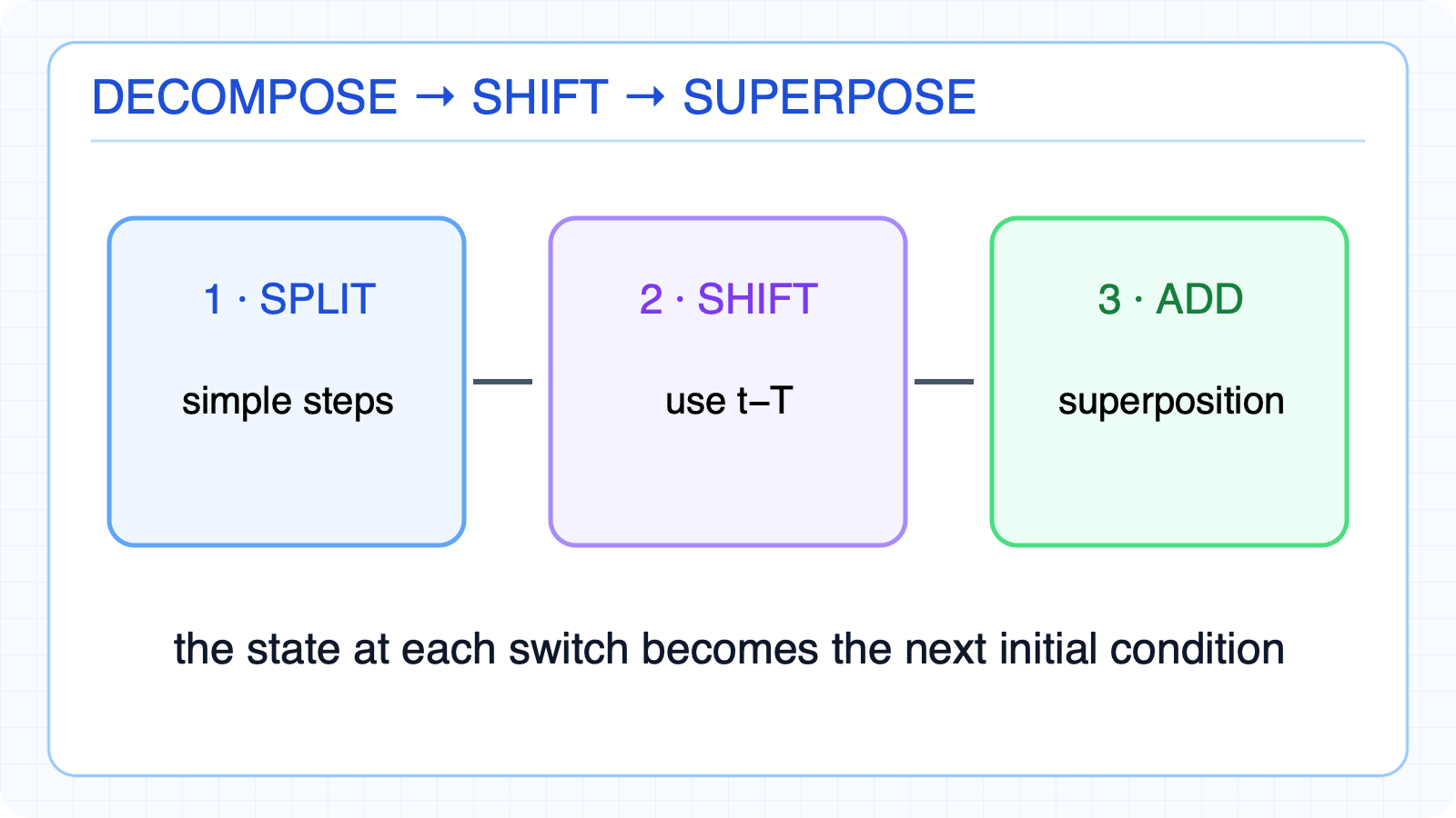
Decompose, time-shift, and add responses with the correct initial state. Decompose a complex input into simple partsDigital clocks and data signals are pulse trainsRC response determines timing delayBrief excitations reveal sensor transientsMedical and power systems use controlled energy pulsesWrite the start time of every componentThe switching state becomes the next initial conditionUse each response only in its valid regionFinish with continuity and limit checksNarration transcript
Pulse inputs appear everywhere in engineering. In digital circuits, clock signals and data buses are essentially streams of pulses. Understanding how RC circuits respond to pulses helps us predict signal integrity and timing delays. In sensor systems, brief pulses are used to excite circuits and measure their transient response. In medical devices like defibrillators, a controlled energy pulse is delivered to the heart. As a preview of what is coming next in this course: when the input is sinusoidal, the analysis changes dramatically. We will use the phasor method and impedance concepts to handle AC steady state circuits. That is the focus of the next major chapter.
5. Pulse-response summary and input preview
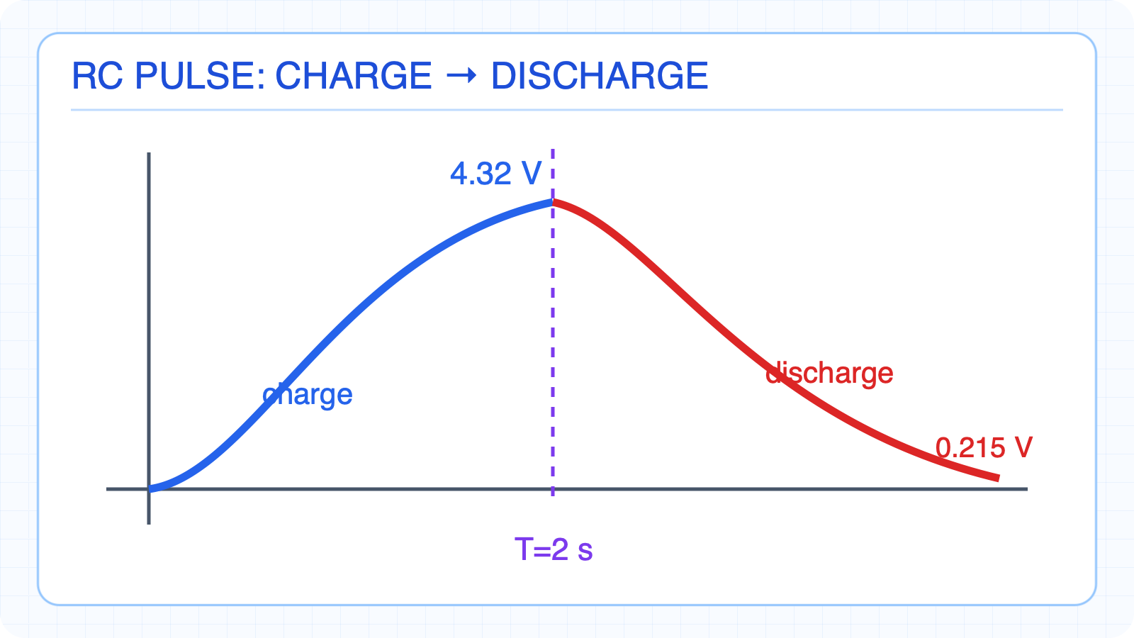
Voltage rises until T and then decays exponentially from that value. The pulse response is built from two stepsBefore T, the RC circuit chargesAfter T, it naturally discharges from vC(T)Here τ=1 s and vC(T)=4.32 VAn exponential input combines source and natural ratesEqual rates produce the repeated-root form t·e(−t/τ)Sinusoidal inputs require phasors and impedanceThe same piecewise logic extends to multiple switchesNext topic: sequential switchingNarration transcript
Let us summarize. We covered three types of inputs today. First, the pulse input: the key technique is superposition of two step responses, one positive at t equals zero and one negative at t equals T. The response has two regions: charging for t less than T, and discharging for t greater than T. Second, exponential inputs: when the source decay rate A differs from one over tau, we get two distinct exponentials. When A equals one over tau, we get the special resonant form t times e to the negative t over tau. Third, we briefly mentioned sinusoidal inputs, which require phasor analysis. Next, we will study sequential switching circuits, where multiple switching events happen at different times.