Circuit Theory 2 · s-Domain node and mesh analysis

#18 KCL and KVL with zero-minus initial states, parallel RC node, and series RL mesh

Write complete RC-node and RL-mesh equations, keeping source directions, initial-state signs and readable fractions.

Question

Reviewed reference card from the existing English final illustrating s-domain circuit equations or the analysis workflow. — Original-video reference. Two circuit diagrams with source-connection or polarity problems use the corresponding rule cards from this same final; the notebook states the complete references and equations.

Apply the zero-minus unilateral Laplace convention to ideal linear constant-parameter lumped circuits, using positive R, C and L. In the parallel RC node example, the top node voltage is measured relative to the common reference node. The current source must be connected between that same reference and top node, injecting current into the top node. Passive resistor and capacitor current references leave the top node toward reference. Define V_0=v_C(0−). Then I_R=V/R, I_C=C[sV−V_0], and KCL gives (1/R+sC)V=I_s+CV_0. Subscript s on I_s or V_s denotes the independent source, not multiplication by the Laplace variable. Thus V=(I_s+CV_0)/(sC+1/R), a sum of the full zero-state input response and zero-input initial-state response. Zero initial voltage gives V=I_s/(sC+1/R); zero input gives V=V_0/(s+1/(RC)). The latter has positive-time natural response V_0 exp(−t/(RC)), with no capacitor-current switching impulse. A driven zero-state response can itself contain transients; the source's forced/natural terminology must not be read as steady-state/transient decomposition. Do not equate zero-minus and zero-plus states across a relevant impulsive switching excitation or double-count an origin impulse and initial-state term. In the series RL example choose one loop current, passive R and L drops, and a source polarity giving a voltage rise along that traversal. Define i_0=i_L(0−) in the same current reference. Then V_s=RI+sLI−Li_0, (R+sL)I=V_s+Li_0, and I=(V_s+Li_0)/(R+sL). For zero input this reduces to i_0/(s+R/L), whose positive-time natural response decays with time constant L/R. In node equations 1/R+sC is admittance in siemens, while I_s and CV_0 are transformed currents in ampere-seconds. In mesh equations R+sL is impedance in ohms, while V_s and Li_0 are transformed voltages in volt-seconds. Initial-state signs and units are part of the model. Larger systems retain dependent-source constraints; ideal voltage sources may require supernodes or modified nodal analysis, and classical mesh analysis assumes a planar circuit. A transfer function is an LTI zero-initial-state relation, not a ratio containing initial-state terms. All nine original final-video frames were inspected. The node example drawing leaves the current-source return open and the ground mark disconnected. The mesh drawing shows the applied source positive at the bottom despite a clockwise current and equations requiring the opposite source rise, and its labels overlap. These two unsuitable figures are not presented as correct circuit diagrams: their notebook roles reuse the readable node-rule and mesh-rule cards from this same final. No corrected source video or new schematic was generated. The node-check arrow crosses its decorative label and the workflow's final s extends across a box border; mathematical content remains visible. Existing single-line raster fractions and these layout/source limitations remain manual teaching QA. The notebook uses complete formatted formulas and explicit references. Source say, MP3 and original cue boundaries are unchanged. This is an unpublished draft, not full human listening, full motion QA or publication approval.

Written solution and narration transcript(shows the full solution)

Below are all the lines written in the notebook together with the full narration transcript.

1. Use Kirchhoff laws in the s-domain
Original-video reference. Two circuit diagrams with source-connection or polarity problems use the corresponding rule cards from this same final; the notebook states the complete references and equations.
Use the ideal linear RLC branch models from lesson 17.
After the unilateral transform, do circuit laws change?
No: keep the same consistent node and loop references.
Kirchhoff current and voltage laws still apply to the lumped-circuit model.
Use transformed currents and voltages throughout each equation.
Keep the zero-minus initial-state source terms as well as the transformed input sources.
Work one parallel RC node and one series RL mesh in the s-domain.
Narration transcript
We now have s-domain models for R, L, and C. The next question is: once the circuit is transformed, do we need new circuit laws? No. Kirchhoff's current law and voltage law still apply. We simply write them using Laplace-domain currents and voltages. The only new pieces are the initial-condition source terms. Today we write one node equation and one mesh equation directly in s.
2. Write node branch currents with the initial voltage
Original-video reference. Two circuit diagrams with source-connection or polarity problems use the corresponding rule cards from this same final; the notebook states the complete references and equations.
Node analysis starts with a reference node.
Define the unknown voltage relative to that reference, with the top node positive.
Use passive branch-current references leaving the top node.
Resistor branch:
$\displaystyle I_{R}\left(s\right)=\frac{V\left(s\right)}{R}$
With initial capacitor voltage measured from top to reference:
$\displaystyle V_{0}=v_{C}\left(0^{-}\right), I_{C}\left(s\right)=s C V\left(s\right)-C V_{0}$
The signed capacitor memory term is a transformed current:
$\displaystyle J_{C}\left(s\right)=-C V_{0}$
Moving that term to the injected-source side changes its sign:
$\displaystyle \left(\frac{1}{R}+s C\right)V\left(s\right)=I_{s}\left(s\right)+C V_{0}$
Narration transcript
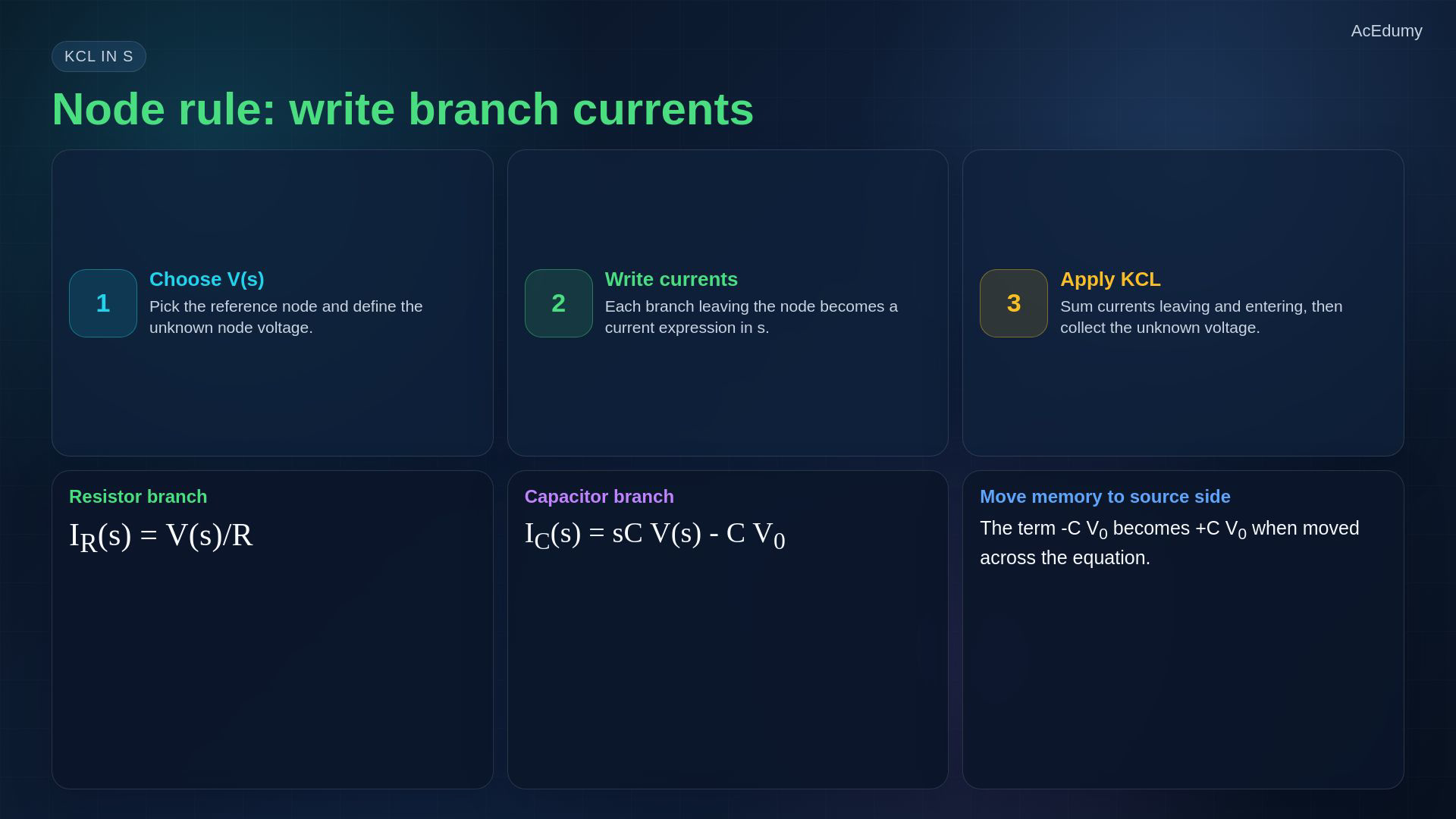
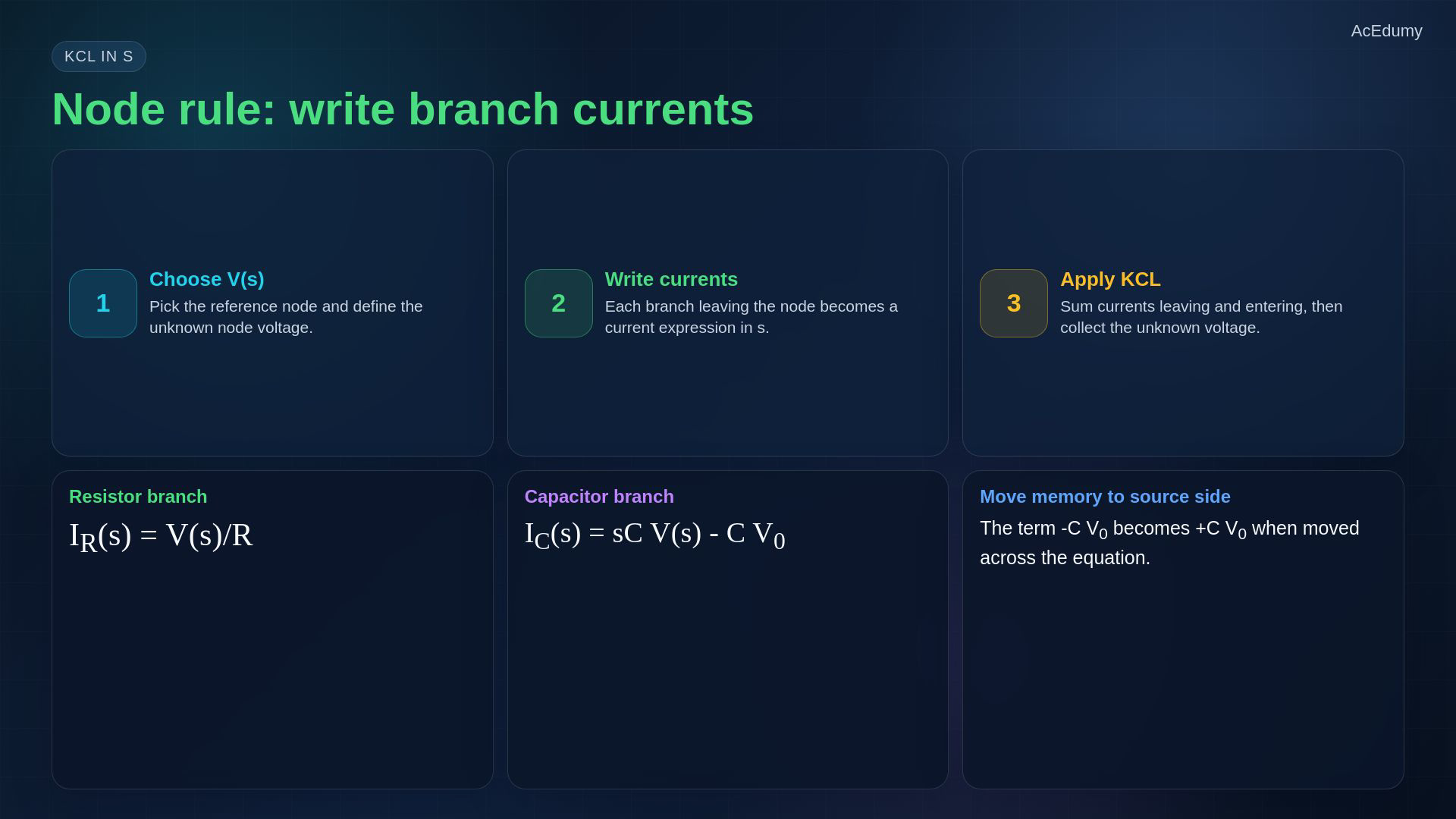
Start with node analysis. Pick the reference node, then define the unknown node voltage V of s. For every branch leaving the node, write the branch current using the s-domain element model. A resistor to ground gives V over R. A capacitor to ground, with initial voltage V naught at the top plate, gives I C of s equals s C V of s minus C V naught. That minus term is the memory term. If we move it to the source side, it becomes plus C V naught.
3. Collect the parallel RC node equation
Original-video reference. Two circuit diagrams with source-connection or polarity problems use the corresponding rule cards from this same final; the notebook states the complete references and equations.
Example: one complete current-source branch feeding a parallel resistor and capacitor.
The source current is directed from the reference node into the top node; subscript s here means source.
Both R and C connect between the top node and the same reference node.
Keep the pre-switch top-to-reference capacitor voltage:
$\displaystyle V_{0}=v_{C}\left(0^{-}\right)$
KCL uses both passive branch currents leaving the node:
$\displaystyle I_{s}\left(s\right)=I_{R}\left(s\right)+I_{C}\left(s\right)$
Substitute complete branch models:
$\displaystyle I_{s}\left(s\right)=\frac{V\left(s\right)}{R}+s C V\left(s\right)-C V_{0}$
Collect the unknown voltage and move the initial term:
$\displaystyle \left(\frac{1}{R}+s C\right)V\left(s\right)=I_{s}\left(s\right)+C V_{0}$
Narration transcript
Here is the node example. A current source I s of s injects current into the node. A resistor and a capacitor go from the node to ground. The capacitor starts with voltage V naught. KCL says: input current equals resistor current plus capacitor current. So I s of s equals V over R plus s C V minus C V naught. Collecting the unknown V gives open parenthesis one over R plus s C close parenthesis V equals I s plus C V naught.
4. Separate zero-state and zero-input terms
Original-video reference. Two circuit diagrams with source-connection or polarity problems use the corresponding rule cards from this same final; the notebook states the complete references and equations.
Check zero initial state separately from zero external input.
For zero initial voltage, this is the complete zero-state input response:
$\displaystyle V_{0}=0, V\left(s\right)=\frac{I_{s}\left(s\right)}{s C+\frac{1}{R}}$
For zero input, the stored state remains:
$\displaystyle I_{s}\left(s\right)=0, \left(s C+\frac{1}{R}\right)V\left(s\right)=C V_{0}$
Divide numerator and denominator by C:
$\displaystyle V\left(s\right)=\frac{V_{0}}{s+\frac{1}{R C}}$
The total is the sum of zero-state and zero-input parts; zero-state does not mean steady-state only.
Narration transcript
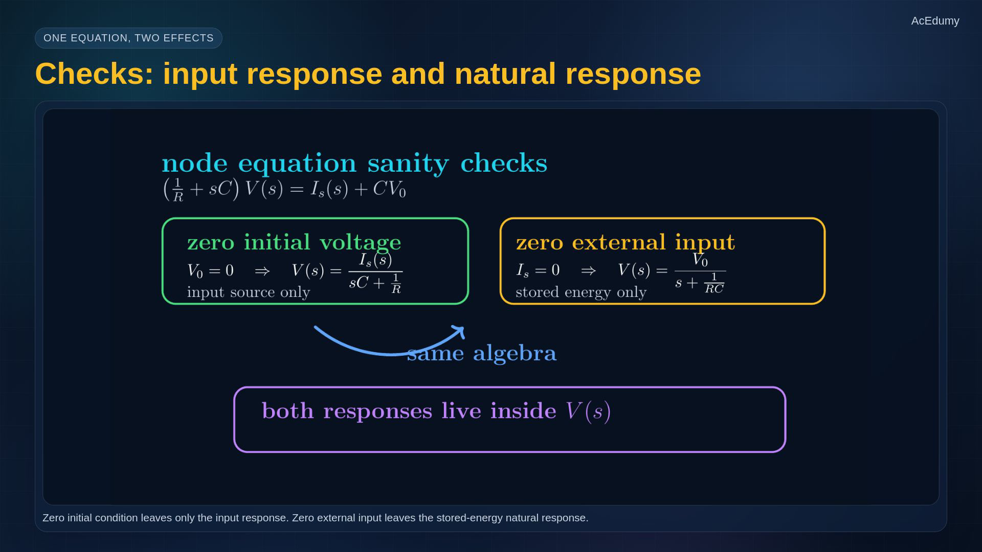
Two quick checks make the equation trustworthy. If the initial voltage V naught is zero, the memory term disappears and only the input source drives the node. If the input source is zero, the stored capacitor energy still drives the natural response. The same equation gives V of s equals V naught over s plus one over R C. So forced response and natural response live together in the same algebra.
5. Write passive branch voltage drops
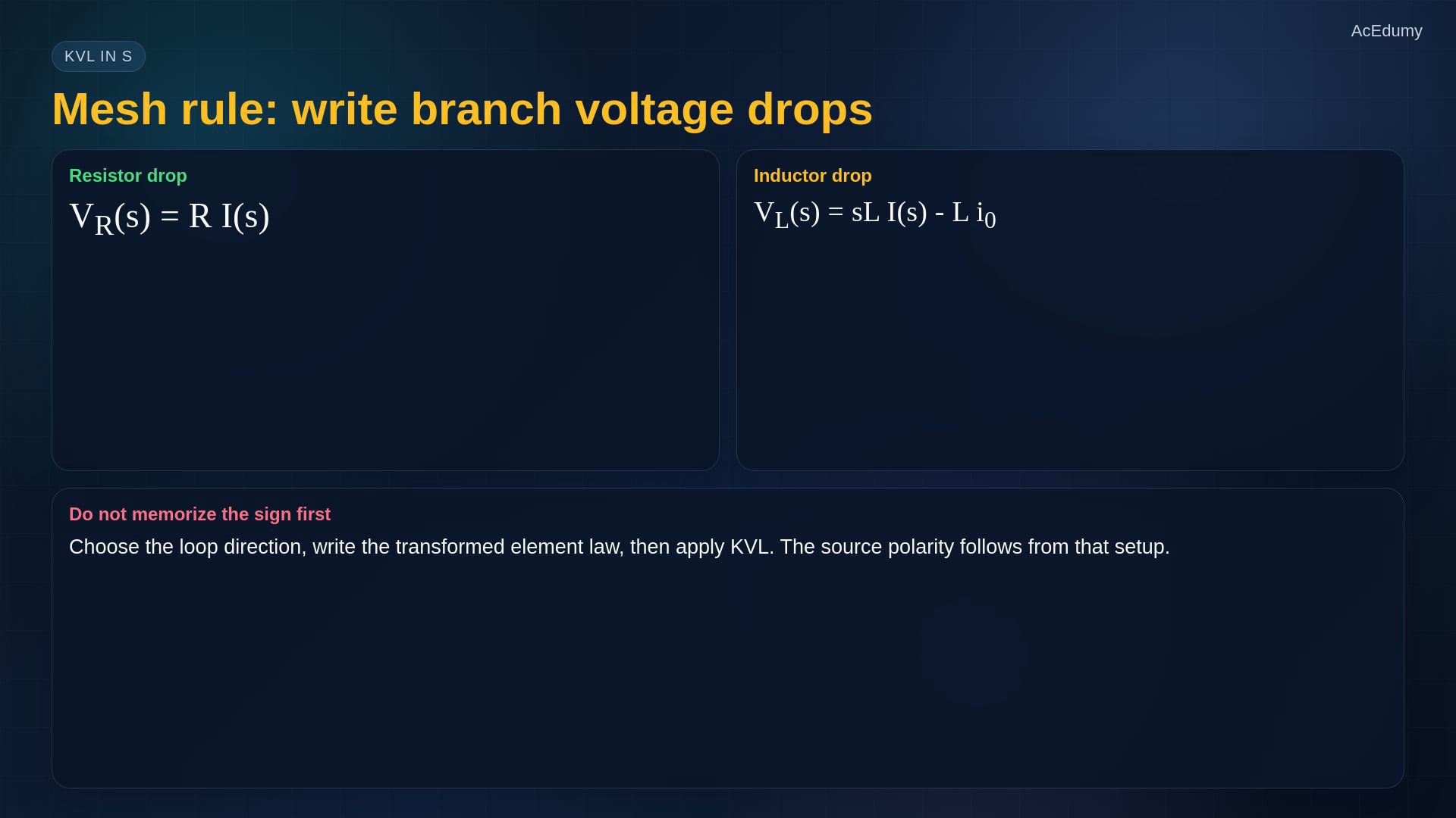
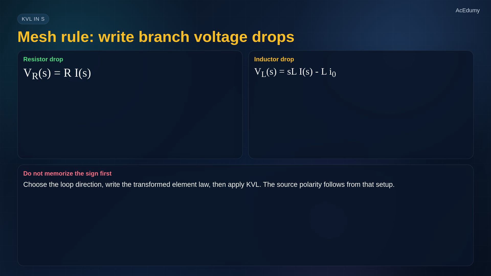
Original-video reference. Two circuit diagrams with source-connection or polarity problems use the corresponding rule cards from this same final; the notebook states the complete references and equations.
Now choose a mesh-current reference and consistent branch voltages.
Traverse the loop in the chosen current direction; define the applied source as a voltage rise.
Use passive voltage drops across the resistor and inductor.
Resistor voltage drop:
$\displaystyle V_{R}\left(s\right)=R I\left(s\right)$
With the initial inductor current in that reference:
$\displaystyle i_{0}=i_{L}\left(0^{-}\right), V_{L}\left(s\right)=s L I\left(s\right)-L i_{0}$
The applied voltage rise equals the sum of the passive drops:
$\displaystyle V_{s}\left(s\right)=V_{R}\left(s\right)+V_{L}\left(s\right)$
Derive the initial-source sign from these references and the derivative rule.
Narration transcript
Now use mesh analysis. Pick a loop current I of s and traverse the loop. Every s-domain branch contributes a voltage drop. A resistor gives R I. An inductor whose current reference matches the loop gives s L I minus L i naught. KVL says the applied source equals the sum of drops. The sign of the initial source is not something to memorize first; it comes from the chosen reference direction and the transformed element law.
6. Collect the series RL mesh equation
Original-video reference. Two circuit diagrams with source-connection or polarity problems use the corresponding rule cards from this same final; the notebook states the complete references and equations.
Example: a series R-L loop driven by a source whose polarity gives a rise along the chosen loop direction.
The signed initial current uses the same inductor and mesh reference:
$\displaystyle i_{0}=i_{L}\left(0^{-}\right)$
KVL with the full initial-current term:
$\displaystyle V_{s}\left(s\right)=R I\left(s\right)+s L I\left(s\right)-L i_{0}$
Move the initial term while collecting current:
$\displaystyle \left(R+s L\right)I\left(s\right)=V_{s}\left(s\right)+L i_{0}$
Divide the entire numerator by the complete impedance:
$\displaystyle I\left(s\right)=\frac{V_{s}\left(s\right)+L i_{0}}{R+s L}$
Narration transcript
For the mesh example, take a series voltage source V s of s, a resistor R, and an inductor L. The initial inductor current i naught points in the mesh direction. KVL gives V s equals R I plus s L I minus L i naught. Collecting I gives open parenthesis R plus s L close parenthesis I equals V s plus L i naught. Therefore I of s equals V s plus L i naught, divided by R plus s L.
7. Transform, collect, solve and invert
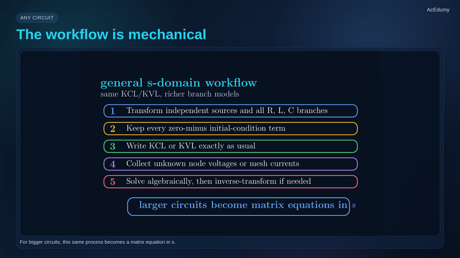
Original-video reference. Two circuit diagrams with source-connection or polarity problems use the corresponding rule cards from this same final; the notebook states the complete references and equations.
A repeatable workflow for ideal linear lumped circuits.
Transform the independent inputs and every branch law; retain any dependent-source constraints.
Keep the zero-minus initial-state terms in the chosen unilateral convention.
Write signed KCL or KVL with consistent references.
Collect the unknown voltages or currents, including any extra source constraints.
Solve algebraically and invert when the positive-time waveform is needed.
Larger systems become matrix equations; ideal voltage sources may require supernodes or modified nodal analysis.
Narration transcript
The general workflow is mechanical. First, transform independent sources and all R, L, C branches into s-domain models. Second, keep every zero-minus initial condition. Third, write KCL or KVL exactly as you would in circuit analysis. Fourth, collect the unknown node voltages or mesh currents. Fifth, solve in algebra and inverse-transform if you need the time waveform. For larger circuits, the same process becomes a matrix equation in s.
8. Check domains, source signs and zero-minus states
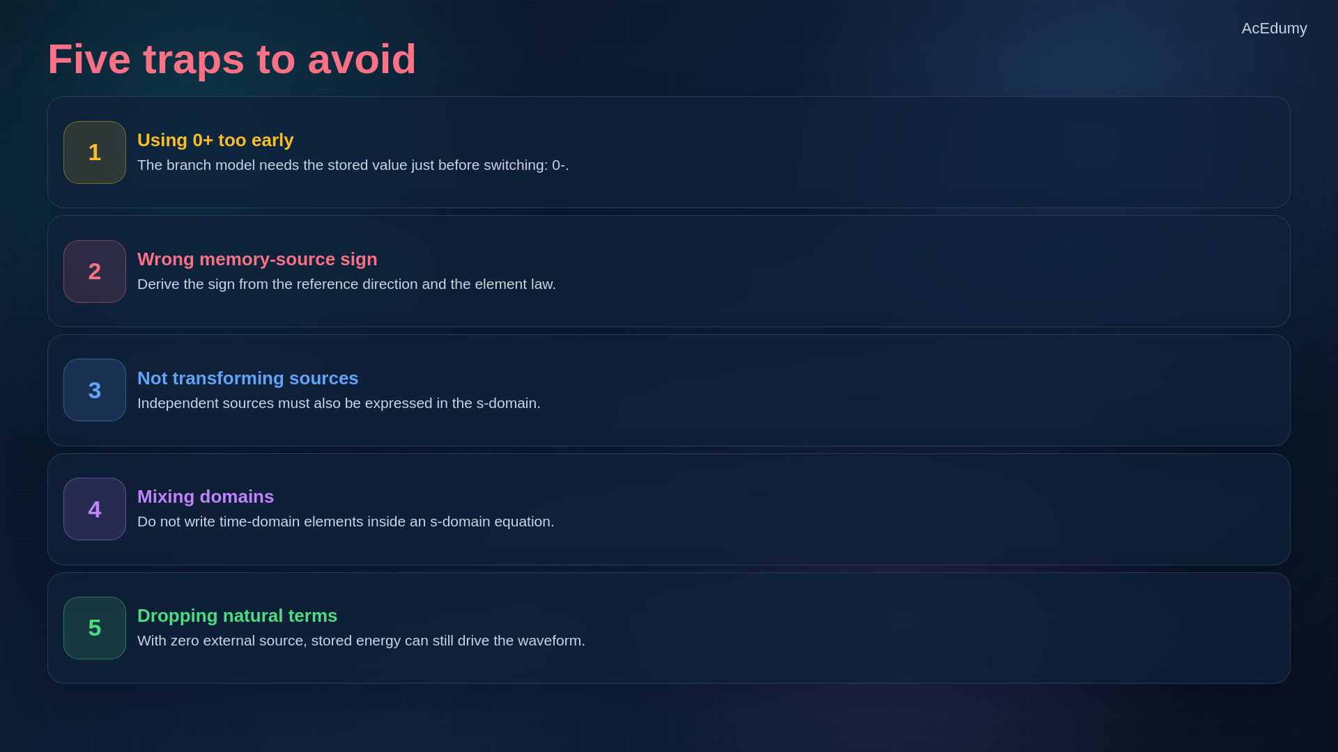
Original-video reference. Two circuit diagrams with source-connection or polarity problems use the corresponding rule cards from this same final; the notebook states the complete references and equations.
Five checks before trusting the transformed circuit.
Do not replace zero minus by zero plus without checking whether the relevant state is continuous.
Derive memory-source signs; do not memorize polarity independently of the reference.
Transform the input source as well as the passive elements.
Keep transformed variables and time-domain quantities clearly distinguished.
Zero external input can still leave a nonzero initial-state response.
Narration transcript
Watch for five traps. Do not use zero plus when the element model needs zero minus. Do not give the memory source the wrong sign. Do not forget that independent sources also transform into the s-domain. Do not mix time-domain elements with s-domain equations. And do not drop natural terms just because the external source is zero; stored energy can be the source.
9. Carry both input and initial-state response
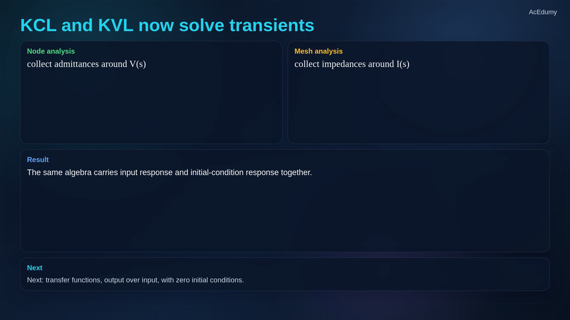
Original-video reference. Two circuit diagrams with source-connection or polarity problems use the corresponding rule cards from this same final; the notebook states the complete references and equations.
Summary: the same circuit laws carry both effects.
Lesson 17 supplies complete RLC branch models.
Insert those models into consistently referenced circuit equations.
For the RC node, the coefficient is an admittance:
$\displaystyle Y_{N}\left(s\right)=\frac{1}{R}+s C$
For the RL mesh, the coefficient is an impedance:
$\displaystyle Z_{M}\left(s\right)=R+s L$
Separate zero-state input response from zero-input initial-state response; add them for the total.
Next: define an LTI transfer function from output over input with zero initial conditions.
Narration transcript
Summary. Lesson seventeen gave us the branch models. This lesson shows how to use them in equations. Node analysis collects admittances around V of s. Mesh analysis collects impedances around I of s. The result contains the input response and the initial-condition response together. Next, we turn these equations into transfer functions: output over input, with zero initial conditions.