#47 Transient Analysis #47 — Parallel RLC and the second-order natural response

Below are all the lines written in the notebook together with the full narration transcript.

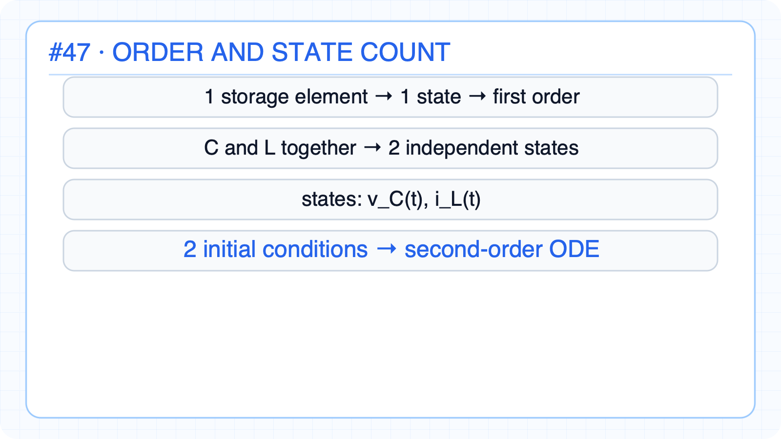
1. 1. Why second order?

   

   One energy-storage element → one state

   A circuit with only C or only L is first order

   C and L together store energy in the same network

   Two independent states: v_C(t) and i_L(t)

   Two independent initial conditions are required

   The natural response obeys a second-order differential equation

   Narration transcript

   In first-order circuits, we had only one energy storage element, either a capacitor or an inductor. That gave us one state variable and one time constant. Now we move to second-order circuits, where a capacitor and an inductor appear together in the same network. That means the circuit can store both electric-field energy and magnetic-field energy. As a result, the natural response is no longer governed by a first-order equation. We now need a second-order differential equation.

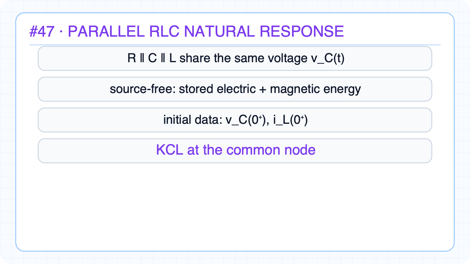
2. 2. Set up the parallel RLC natural response

   

   R, C, and L are in parallel between the same two nodes

   All three branches share v_C(t)

   The inductor branch contributes the state i_L(t)

   There is no independent source: stored energy drives the motion

   Initial data: v_C(0⁺) and i_L(0⁺)

   KCL at the top node will produce one governing equation

   Narration transcript

   Consider the parallel R L C circuit. The resistor, inductor, and capacitor all share the same node voltage. We call that capacitor voltage v c of t. The inductor current i L of t is the second state variable. Because two independent initial conditions are needed, typically v c of zero and i L of zero, this is a second-order system. Our goal is to write one differential equation that describes the natural response.

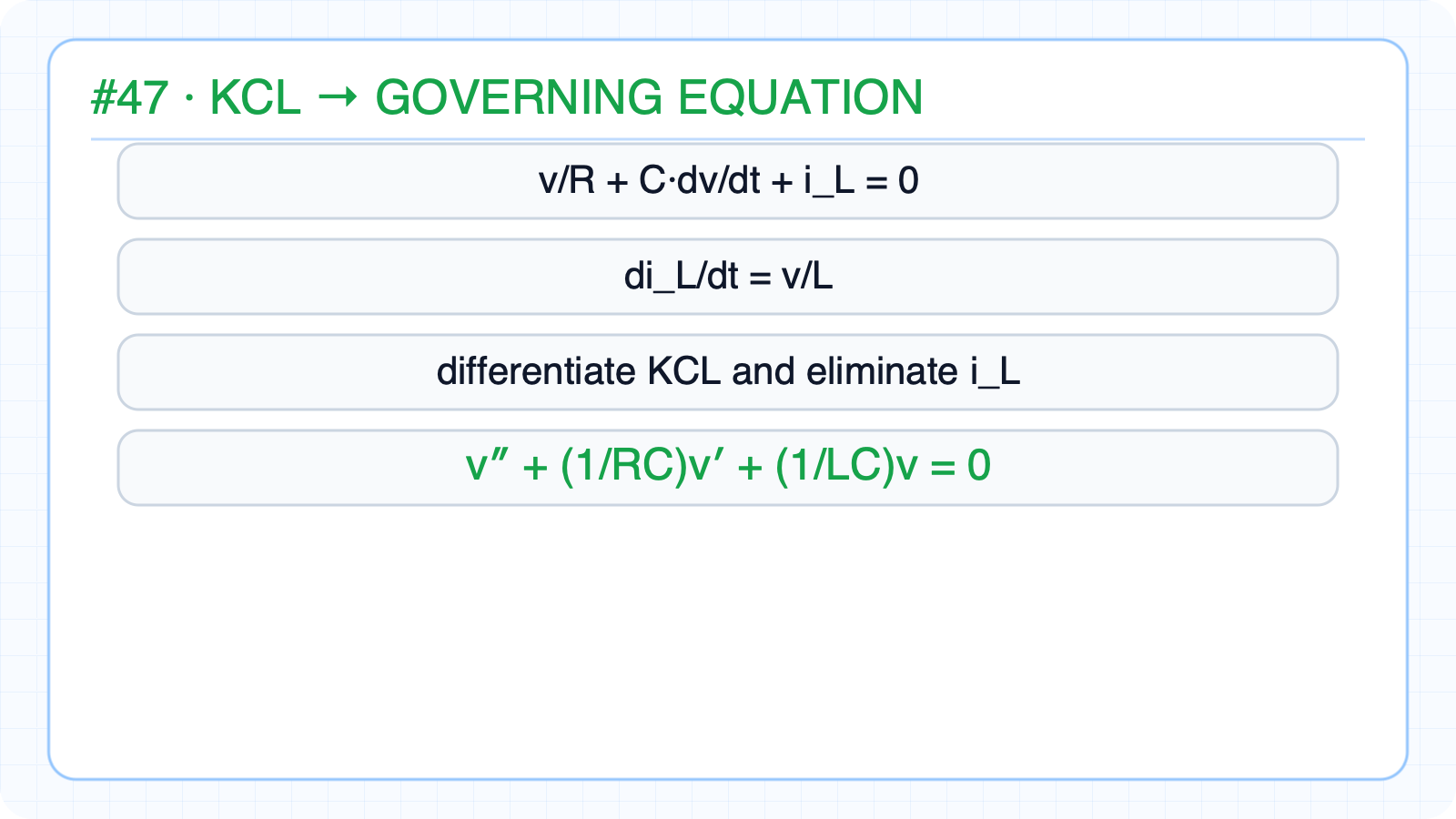
3. 3. Derive the second-order equation from KCL

   

   Write KCL at the top node for the natural response

   v/R + C·dv/dt + i_L = 0

   Inductor law: v=L·di_L/dt

   di_L/dt=v/L

   Differentiate the KCL equation with respect to time

   Replace the derivative of i_L by v/L

   d²v_C/dt² +(1/RC)dv_C/dt +(1/LC)v_C=0

   Narration transcript

   Apply Kirchhoff's current law at the top node. The resistor current plus the capacitor current plus the inductor current must sum to zero for the natural response. Using element laws, the resistor current is v over R, the capacitor current is C times d v over d t, and the inductor relation is v equals L times d i L over d t. If we differentiate the node equation and eliminate the inductor current, we obtain the governing equation: d squared v c over d t squared, plus one over R C times d v c over d t, plus one over L C times v c equals zero. This is the standard second-order homogeneous equation for the parallel R L C natural response.

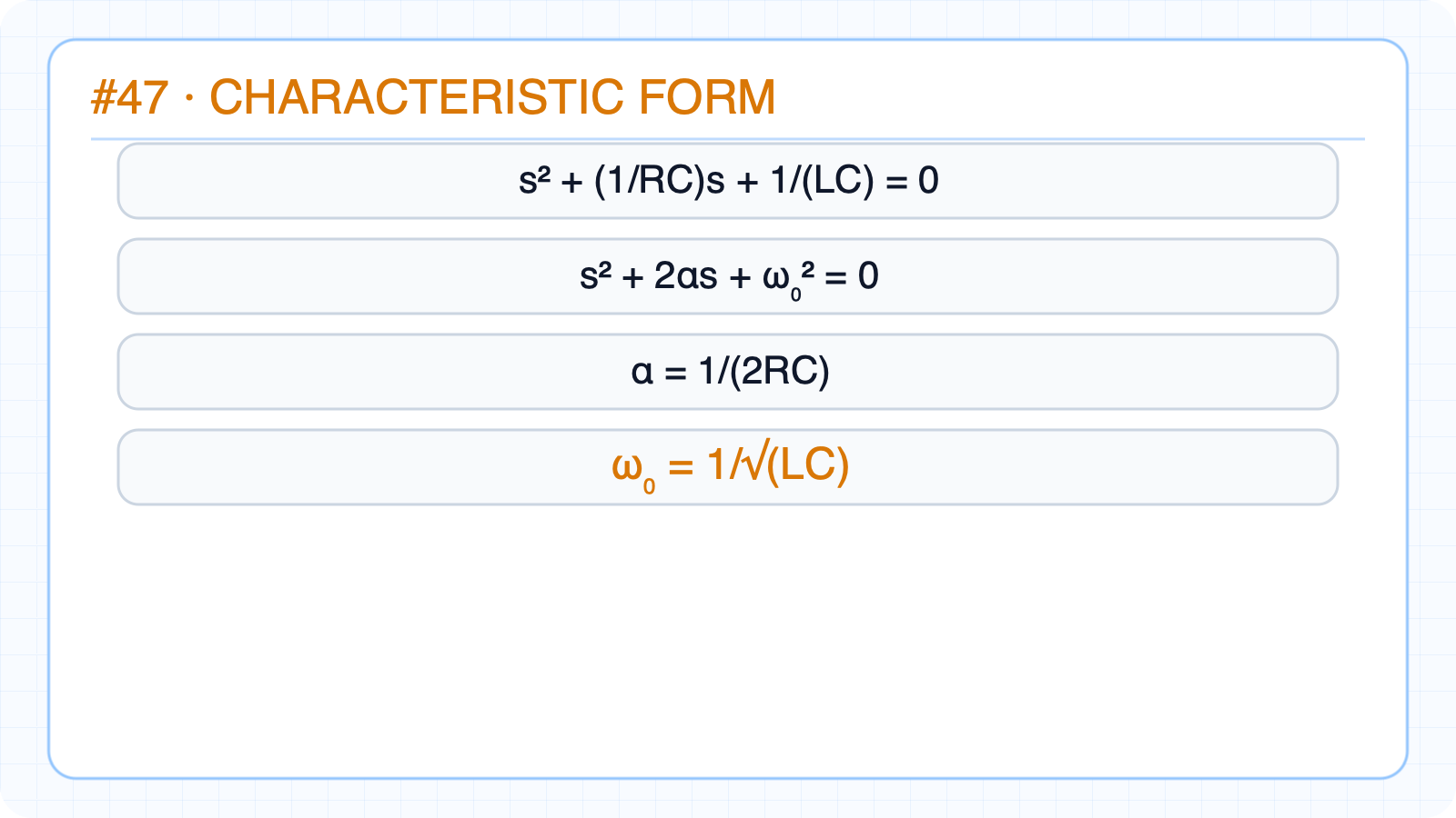
4. 4. Characteristic equation and parameters

   

   Try the exponential solution v_C(t)=Ke^st

   s² +(1/RC)s +1/(LC)=0

   Standard form: s²+2αs+ω₀²=0

   α=1/(2RC) [s⁻¹]

   ω₀=1/√(LC) [rad/s]

   α measures damping; ω₀ is the undamped natural frequency

   The comparison of α and ω₀ selects the response type

   Narration transcript

   Now compare this equation with the standard form s squared plus two alpha s plus omega zero squared equals zero. From that comparison, alpha equals one over two R C, and omega zero equals one over square root of L C. These two parameters control the behavior of the circuit. Alpha represents damping. Omega zero is the undamped natural frequency. The relationship between alpha and omega zero tells us what kind of response we will see.

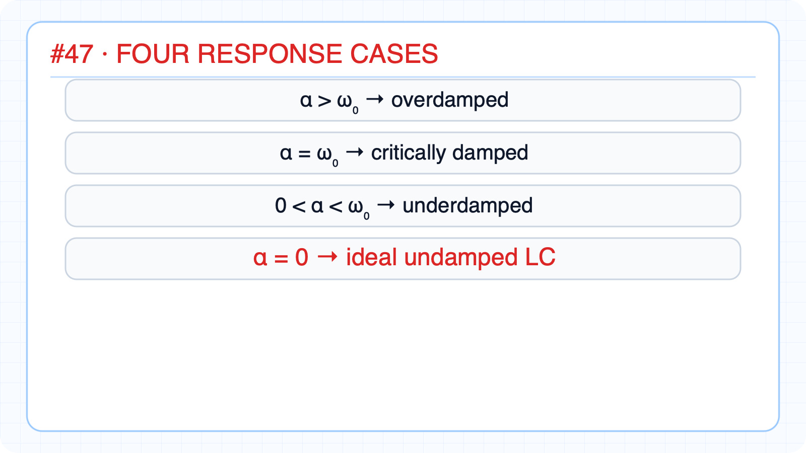
5. 5. Classify the four damping cases

   

   The relation between α and ω₀ controls the roots

   α>ω₀: overdamped, two real roots

   α=ω₀: critically damped, repeated root

   0<α<ω₀: underdamped, complex-conjugate roots

   α=0: ideal undamped LC oscillation

   The first two cases do not oscillate

   In the last two, energy moves between C and L

   Narration transcript

   There are four important cases. If alpha is greater than omega zero, the response is overdamped: no oscillation, but a slow return with two real roots. If alpha equals omega zero, the response is critically damped: the fastest non-oscillatory return. If alpha is less than omega zero, the response is underdamped: oscillation with an exponentially decaying envelope. Finally, if alpha equals zero, we get the ideal undamped L C case: sustained oscillation. In the next two lessons, we will study these cases separately so each one stays short and clear.

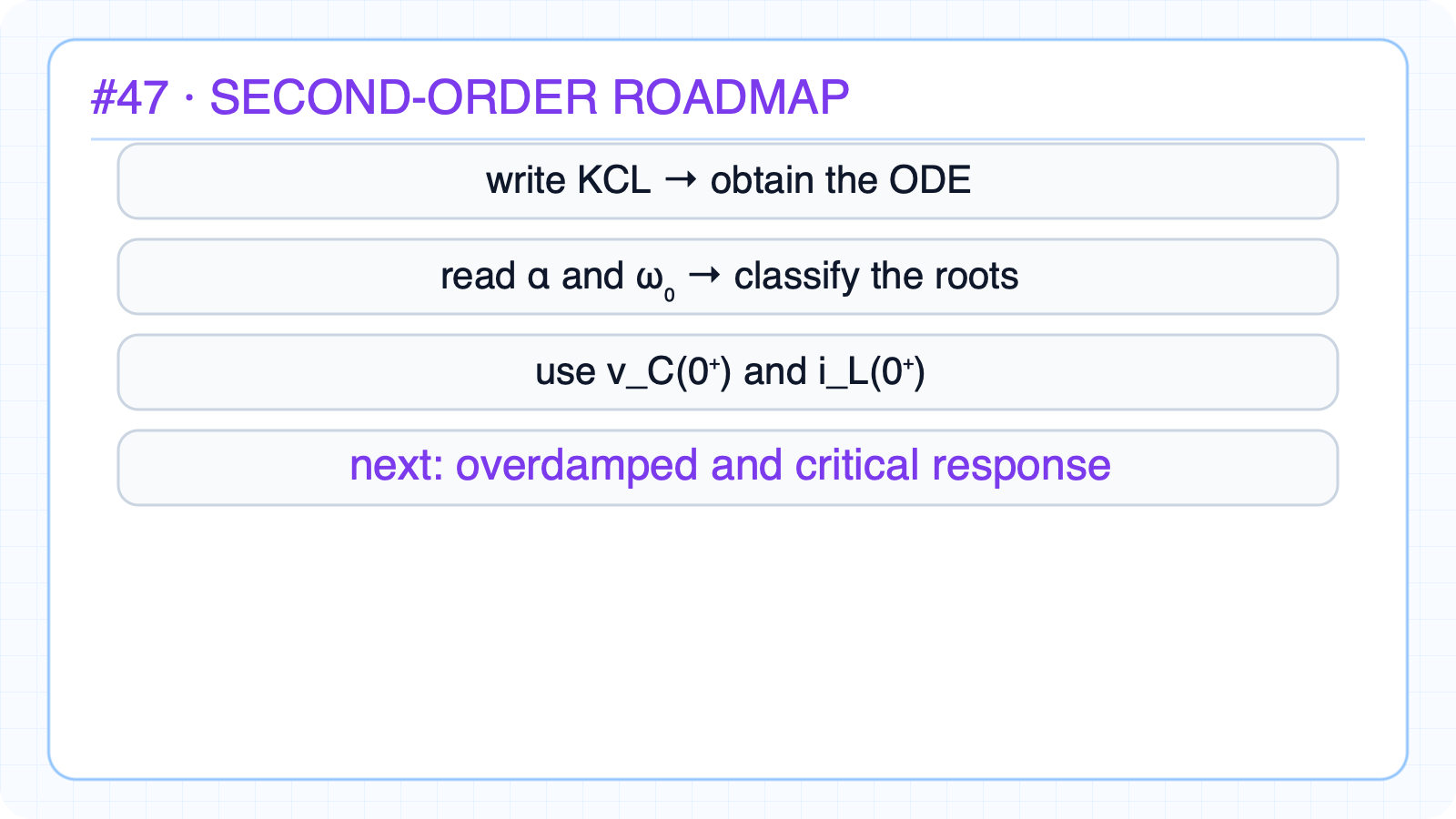
6. 6. Second-order solution roadmap

   

   Use v_C(t) as the shared variable of the parallel RLC

   Write KCL, differentiate, and eliminate i_L

   v″+(1/RC)v′+(1/LC)v=0

   Read α and ω₀ from the equation

   Use two initial conditions to determine two constants

   The comparison α ? ω₀ selects the response form

   Next: overdamped and critically damped response

   Narration transcript

   Let us summarize. A parallel R L C circuit is a second-order system because it contains both a capacitor and an inductor. Its natural response is governed by a second-order differential equation. The key parameters are alpha, the damping factor, and omega zero, the undamped natural frequency. By comparing alpha and omega zero, we classify the response into overdamped, critically damped, underdamped, or undamped. Next lesson: overdamped and critically damped responses.