#51 Transient Analysis #51 — Series-RLC natural response and duality

Below are all the lines written in the notebook together with the full narration transcript.

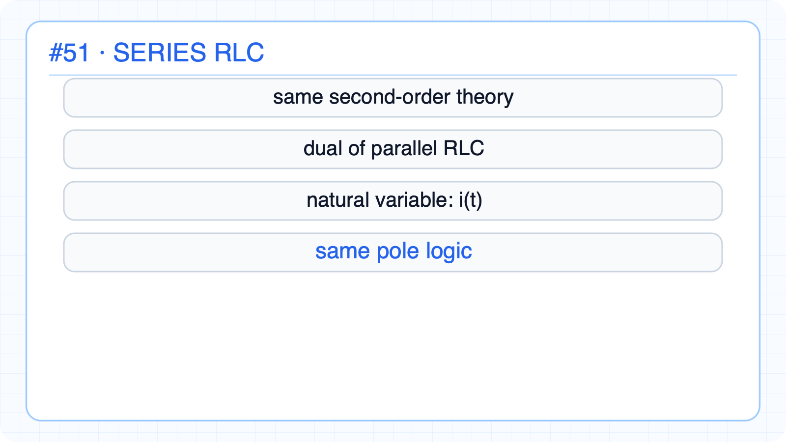
1. 1. Connect series RLC to parallel RLC

   

   Series RLC is not a new theory

   The same second-order behavior appears in the dual circuit

   Voltage is often the natural variable in the parallel form

   Current i(t) is often the natural variable in the series form

   The same current passes through every element

   The circuit form changes; the pole logic does not

   Narration transcript

   So far, we focused on the parallel R L C form. Now we switch to the series R L C circuit. This is not a new theory. It is the same second-order behavior seen through the dual circuit. The key difference is the natural variable we watch. In the series form, current is often the cleanest state variable.

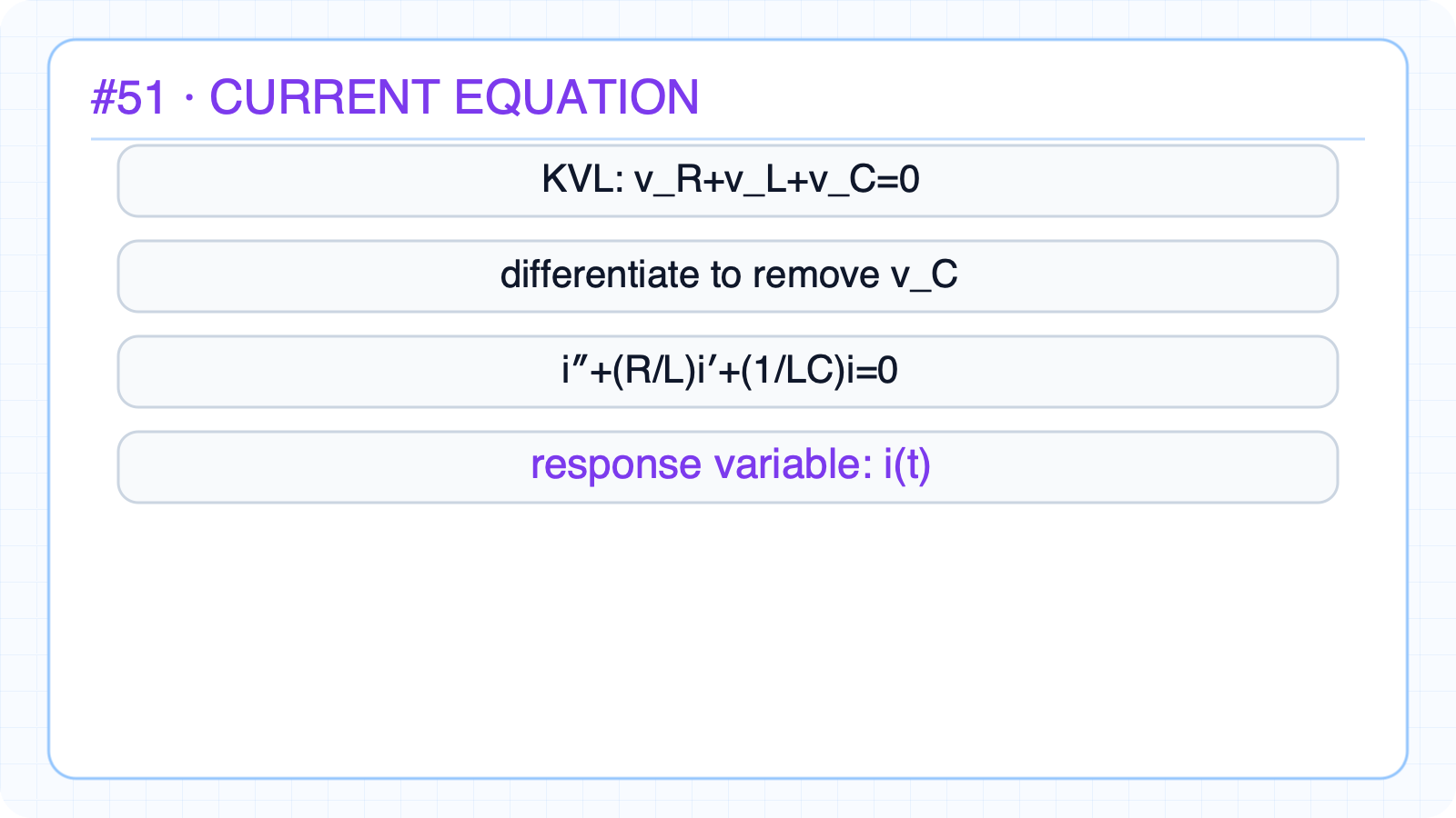
2. 2. Build the series-RLC natural-response equation

   

   Apply KVL to a source-free series RLC loop

   $v_{\mathrm{R}}+v_{\mathrm{L}}+v_{\mathrm{C}}=0$

   v_R=Ri and v_L=L di/dt

   Differentiate to eliminate capacitor voltage

   d²i/dt²+(R/L)di/dt+(1/LC)i=0

   This is the standard homogeneous second-order equation

   Response variable: series current i(t)

   Narration transcript

   For the series R L C natural response, the same current flows through the resistor, inductor, and capacitor. If we write the loop equation and eliminate the capacitor voltage, we obtain the standard second-order equation for current: d squared i over d t squared plus R over L times d i over d t plus one over L C times i equals zero. So the series circuit has the same second-order structure as the parallel circuit.

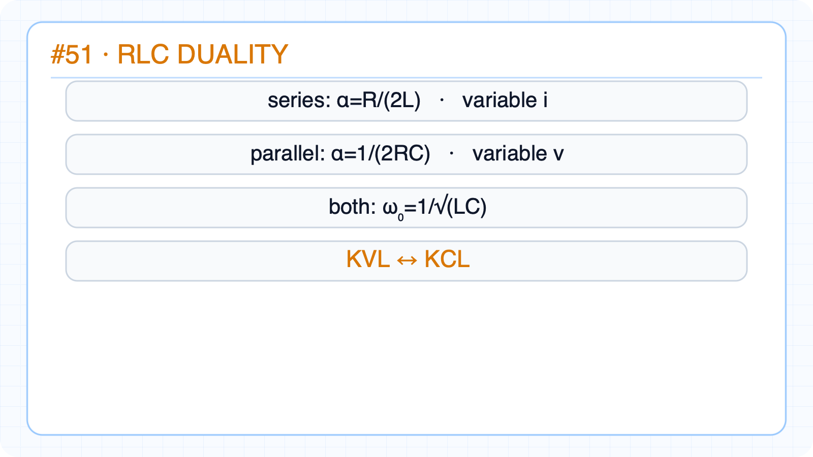
3. 3. Build the series-parallel RLC duality

   

   Series RLC

   $\alpha_{\mathrm{s}}=R/(2L)$

   ω₀=1/√(LC)

   main variable i · loop law KVL

   Parallel RLC

   α_p=1/(2RC)

   main variable v · node law KCL

   ω₀ is the same in both circuits

   Narration transcript

   The parameters also keep the same meaning. For series R L C, alpha equals R over 2 L, and omega zero equals one over square root of L C. Compare that with the parallel form, where alpha equals one over 2 R C. So the natural frequency stays the same, but the damping factor changes because the resistor enters the model differently. Current replaces voltage as the main response variable, and K V L replaces K C L. That is the core duality.

4. 4. Classify a series-RLC example

   

   $R=1 \Omega, L=1 H, C=0.25 F$

   $\alpha=R/(2L)=0.5 s⁻¹$

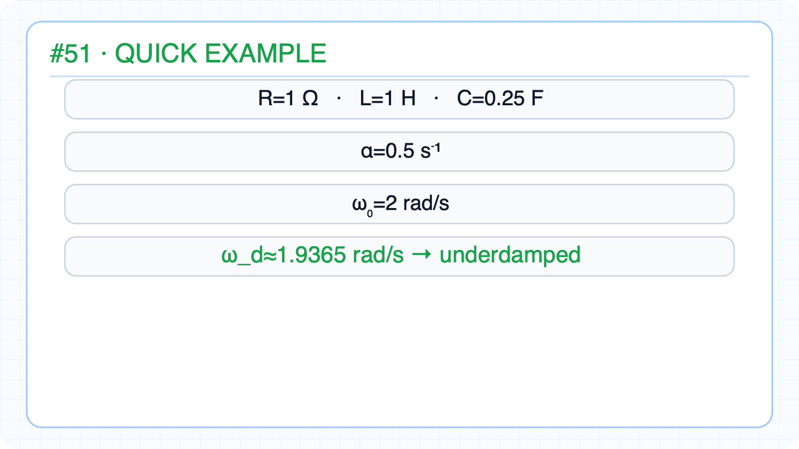
   ω₀=1/√(LC)=2 rad/s

   Because α<ω₀, the response is underdamped

   ω_d=√(ω₀²−α²)=√3.75≈1.9365 rad/s

   $i_{\mathrm{n}}=e^{-0.5t}[B₁\cos (1.9365t)+B₂\sin (1.9365t)]$

   Initial conditions determine B₁ and B₂

   Narration transcript

   Let us test one quick example. Suppose R equals 1 ohm, L equals 1 henry, and C equals one fourth farad. Then alpha becomes one over two, while omega zero becomes two radians per second. Since alpha is smaller than omega zero, the circuit is underdamped. So we expect oscillation under a decaying envelope.

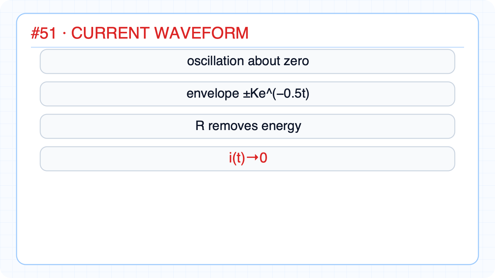
5. 5. Interpret the series-current waveform

   

   Current oscillates about zero

   Resistance removes energy each cycle

   Envelope: ±Ke^−0.5t

   Oscillation rate: ω_d≈1.9365 rad/s

   For the natural response, i(t)→0

   α sets decay; ω_d sets oscillation

   The physical interpretation matches parallel RLC

   Narration transcript

   Here is the resulting current behavior. The series current oscillates, but the envelope shrinks because resistance removes energy from the system. The final natural response still goes to zero, yet the path depends on alpha and omega zero exactly as before. The circuit form changed, but the second-order logic stayed the same.

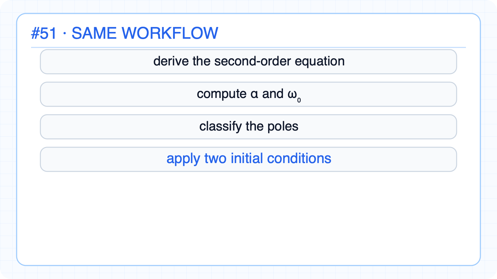
6. 6. Summarize the series-RLC natural response

   

   Series RLC is the dual form of parallel RLC

   i″+(R/L)i′+(1/LC)i=0

   α=R/(2L), ω₀=1/√(LC)

   The over-, critical-, under-, and undamped cases all remain

   Initial conditions determine two constants

   The second-order workflow stays the same when the circuit changes

   Next: focused second-order problem solving

   Narration transcript

   Let us summarize. Series R L C is the dual of parallel R L C. Its natural response for current satisfies a second-order differential equation with alpha equal to R over 2 L and omega zero equal to one over square root of L C. The same four cases still exist: overdamped, critical, underdamped, and undamped. Next lesson, we use these ideas in focused second-order problem solving.