#08 Dipole geometry, far-field path linearization, the vector-potential line integral, and the short dipole's sine-theta pattern

Below are all the lines written in the notebook together with the full narration transcript.

1. 1. Recall the far-field shortcut from d07

   

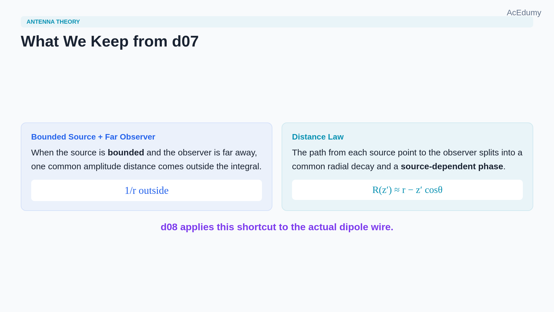
   In the last lesson, far field meant one specific simplification route.

   A bounded source seen from far enough away could share one common amplitude distance, while the remaining source dependent phase stayed inside the integral.

   Now we keep that same logic, but the source is no longer a point.

   The dipole itself becomes the bounded source we have to evaluate.

   Narration transcript

   In the last lesson, far field meant one specific simplification route. A bounded source seen from far enough away could share one common amplitude distance, while the remaining source dependent phase stayed inside the integral. Now we keep that same logic, but the source is no longer a point. The dipole itself becomes the bounded source we have to evaluate.

2. 2. Set up the z-axis dipole and observer geometry

   

   Place a thin dipole on the z axis and keep the observer at spherical direction r, theta, phi.

   Each current element at position z prime contributes to the observer through a slightly different path length.

   So the dipole is still bounded, but it is not collapsed.

   The real question is how to keep the geometry readable without carrying the exact path law everywhere.

   Narration transcript

   Place a thin dipole on the z axis and keep the observer at spherical direction r, theta, phi. Each current element at position z prime contributes to the observer through a slightly different path length. So the dipole is still bounded, but it is not collapsed. The real question is how to keep the geometry readable without carrying the exact path law everywhere.

3. 3. Linearize R(z′) in the far field

   

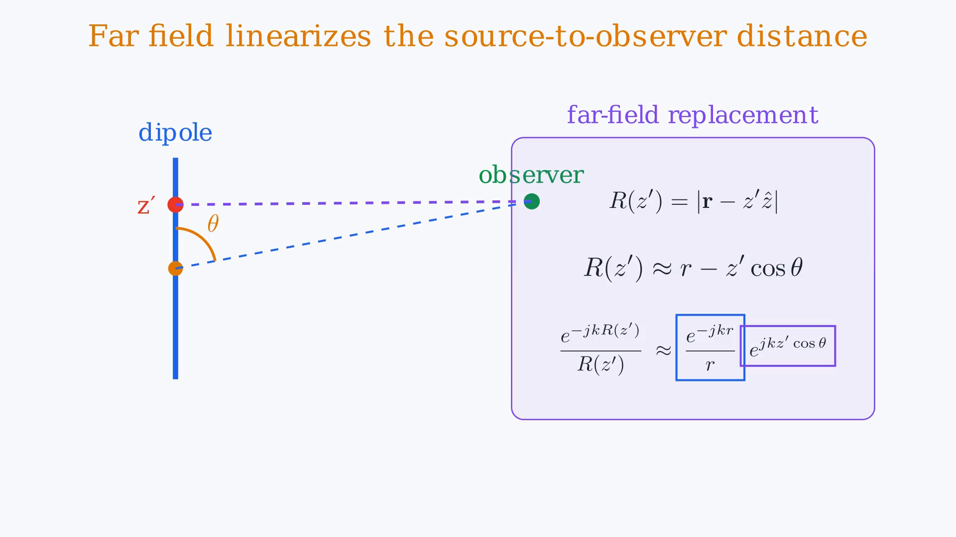
   That is exactly where the far-field approximation enters.

   The exact distance from a source point to the observer is written as R(z′).

   In the far field we replace that exact law by r − z′cos(theta), and we pull 1/R outside as 1/r.

   So amplitude becomes common, while phase still remembers where the source point sits along the wire.

   Narration transcript

   That is exactly where the far-field approximation enters. The exact distance from a source point to the observer is written as R of z prime. In the far field we replace that exact law by r minus z prime cosine theta, and we pull one over big R outside as one over r. So amplitude becomes common, while phase still remembers where the source point sits along the wire.

4. 4. Reduce the vector potential to a dipole line integral

   

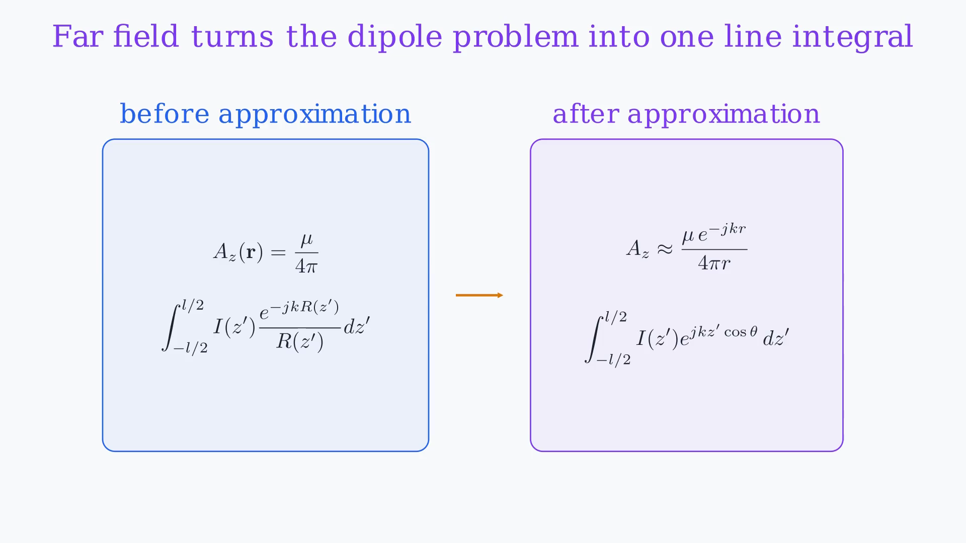
   Once that shortcut is applied inside the vector potential, the dipole problem becomes a line current integral.

   The common factor e⁽−jkr)/r sits outside, because every source point shares the same far observer.

   Inside the integral we keep the current distribution and the source dependent phase term e⁽jkz′cos(theta)).

   That remaining integral is the part that builds the pattern.

   Narration transcript

   Once that shortcut is applied inside the vector potential, the dipole problem becomes a line current integral. The common factor e to the minus j k r over r sits outside, because every source point shares the same far observer. Inside the integral we keep the current distribution and the source dependent phase term e to the plus j k z prime cosine theta. That remaining integral is the part that builds the pattern.

5. 5. Derive the short-dipole E_theta far field

   

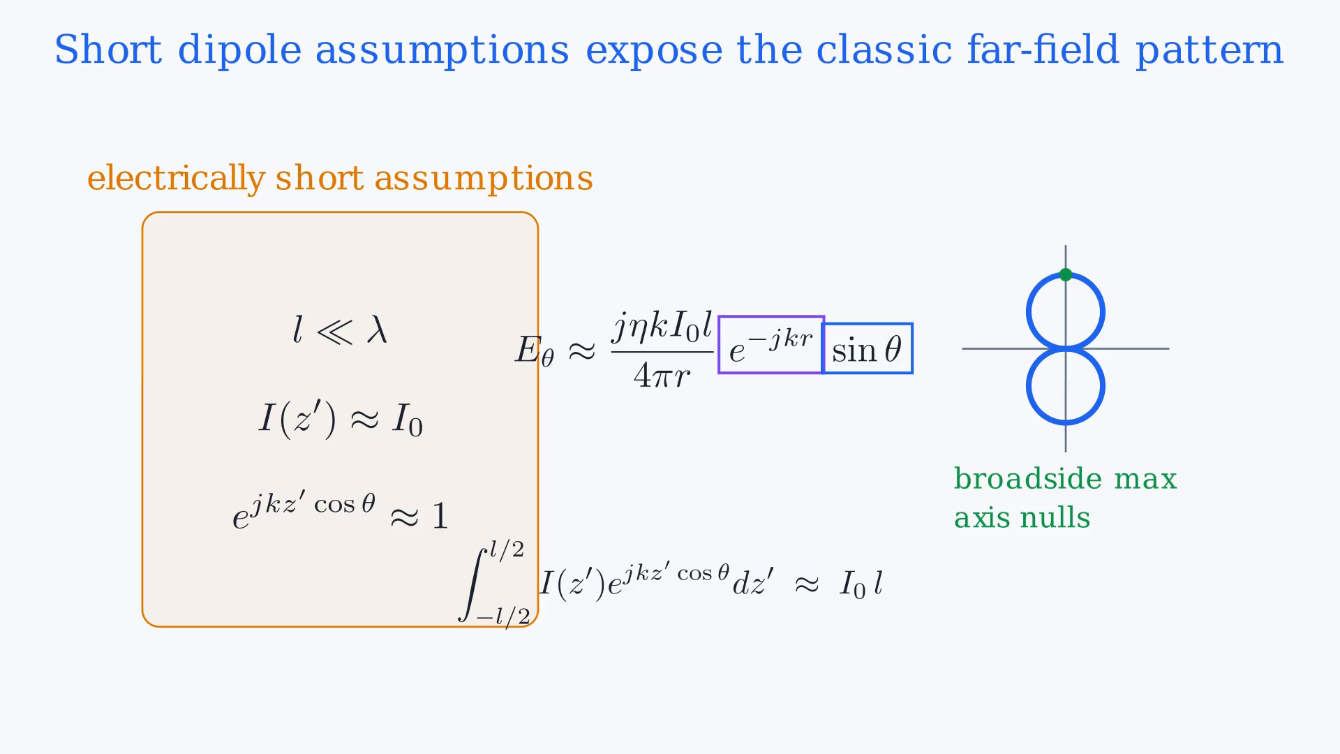
   For the electrically short dipole, we make one more simplification.

   The current is treated as approximately uniform over the short length, and the phase variation across that tiny wire is also mild.

   Then the integral reduces to I₀l.

   After the usual field conversion, the far field becomes E_theta proportional to [e⁽−jkr)/r]sin(theta), with the strength factor jηkI₀l/(4π).

   Narration transcript

   For the electrically short dipole, we make one more simplification. The current is treated as approximately uniform over the short length, and the phase variation across that tiny wire is also mild. Then the integral reduces to I zero times l. After the usual field conversion, the far field becomes E theta proportional to e to the minus j k r over r times sine theta, with the strength factor j eta k I zero l over four pi.

6. 6. Read the nulls and maximum of the sine-theta pattern

   

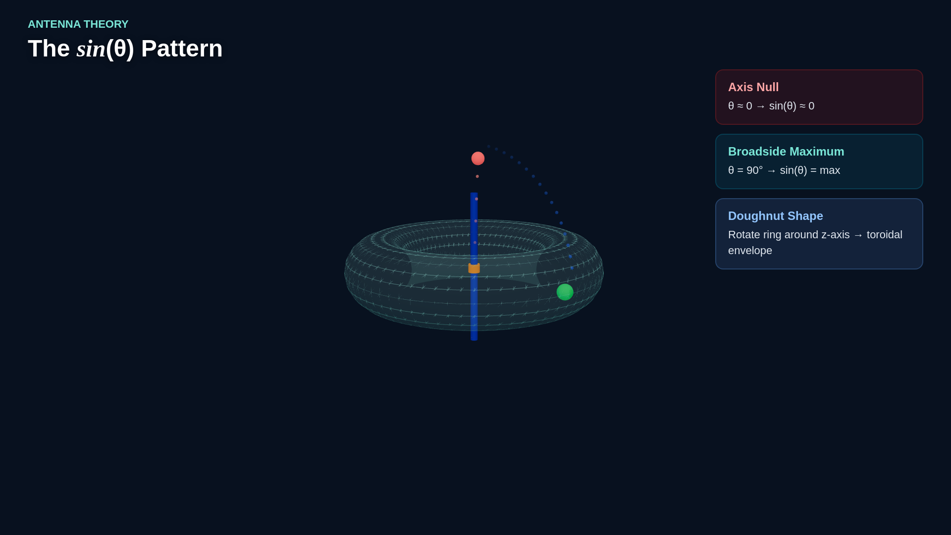
   That sin(theta) term is the pattern story.

   Along the dipole axis, theta is near zero, so sin(theta) is also near zero and the radiation fades.

   At broadside, theta approaches 90°, sin(theta) reaches its maximum, and the dipole radiates most strongly.

   This is the classic doughnut shaped dipole pattern in far field form.

   Narration transcript

   That sine theta term is the pattern story. Along the dipole axis, theta is near zero, so sine theta is also near zero and the radiation fades. At broadside, theta approaches ninety degrees, sine theta reaches its maximum, and the dipole radiates most strongly. This is the classic doughnut shaped dipole pattern in far field form.

7. 7. Summarize spreading, phase, and directivity

   

   So the short dipole far field can be read in three layers.

   1/r gives the geometric spreading.

   e⁽−jkr) gives the propagation phase.

   And sin(theta) gives the directional strength that turns the dipole into a pattern rather than a uniform radiator.

   Narration transcript

   So the short dipole far field can be read in three layers. One over r gives the geometric spreading. E to the minus j k r gives the propagation phase. And sine theta gives the directional strength that turns the dipole into a pattern rather than a uniform radiator.

8. 8. Prepare for stationary phase with an extended source

   

   This lesson worked because the source was still finite and bounded.

   In the next lesson, once the source becomes much more extended, the same shortcut stops being the natural first move.

   That is where stationary phase comes back into the story.

   Narration transcript

   This lesson worked because the source was still finite and bounded. In the next lesson, once the source becomes much more extended, the same shortcut stops being the natural first move. That is where stationary phase comes back into the story.

Source video: Antenna Theory #08 | Dipole Far-Field Solution | Short Dipole Radiation (3:37)