Signals and Systems · Normalization
#23 Signals & Systems #23 | Fourier Series Properties - Square Wave, Derivative Trick & Gibbs
Corrected solution notes. The audio is the original recording and may contain errors or incomplete phrases. Where they differ, use the corrected written solution.
Question
Corrected solution notes. The audio is the original recording and may contain errors or incomplete phrases. Where they differ, use the corrected written solution. Signals & Systems #23 | Fourier Series Properties - Square Wave, Derivative Trick & Gibbs
Written solution and narration transcript(shows the full solution)
Below are all the lines written in the notebook together with the full narration transcript.
1. Normalization
Corrected solution notes. The audio is the original recording and may contain errors or incomplete phrases. Where they differ, use the corrected written solution.If synthesis has prefactor C1 and analysis prefactor C2, use C1C2=1/T.This notebook uses synthesis prefactor one and analysis prefactor 1/T. Do not mix coefficients from different conventions.Narration transcript
In our last two lessons, we introduced the Fourier Series and derived the analysis equations for finding coefficients. Today we explore key properties that make working with Fourier Series much more powerful. Let's start with an important bookkeeping detail. Different textbooks use different scaling conventions. If we write the synthesis as C1 times the sum of X k e to the j k omega zero t, and the analysis as C2 times the integral of x of t e to the minus j k omega zero t, the only requirement is that C1 times C2 equals one over T. In Oppenheim's convention, C1 equals one and C2 equals one over T. In Haykin's convention, the factors are swapped. Both are correct.
2. Differentiation
Differentiation multiplies X[k] by jkω0; the nth derivative multiplies by (jkω0)n under appropriate classical or distributional assumptions.Recover nonzero-index coefficients by division; the lost DC coefficient must be computed separately. Positive and negative k have opposite phase shifts.Narration transcript
Here's one of the most powerful Fourier Series properties: differentiation. If x of t is a periodic signal with Fourier coefficients X sub k, then the derivative y of t equals d x over d t has coefficients Y sub k equals j k omega zero times X sub k. Each coefficient gets multiplied by j times k times the fundamental frequency. The j introduces a 90-degree phase shift, and the factor k means higher harmonics are amplified more. For the nth derivative, we raise the factor to the nth power: Y sub k equals j k omega zero, to the n, times X sub k. More importantly, this property works in reverse. If we know the coefficients of a derivative, we can find the original signal's coefficients by dividing by j k omega zero.
3. Impulse train
A unit impulse repeated every T seconds has X[k]=1/T for all integer k.Interpret the infinite synthesis as a periodic distribution, not an ordinary pointwise sum.Narration transcript
Let's find the Fourier coefficients of a fundamental signal: the periodic impulse train. Delta T of t is the sum of delta functions spaced T seconds apart, from minus infinity to plus infinity. Using the analysis equation, X sub k equals one over T times the integral over one period of delta of t times e to the minus j k omega zero t dt. The sifting property extracts the exponential at t equals zero, giving e to the zero, which is just one. Therefore X sub k equals one over T for all k. Every single coefficient has the same value. This gives us a beautiful identity: the periodic impulse train equals one over T times the sum of e to the j k omega zero t.
4. Flat magnitude is not unique
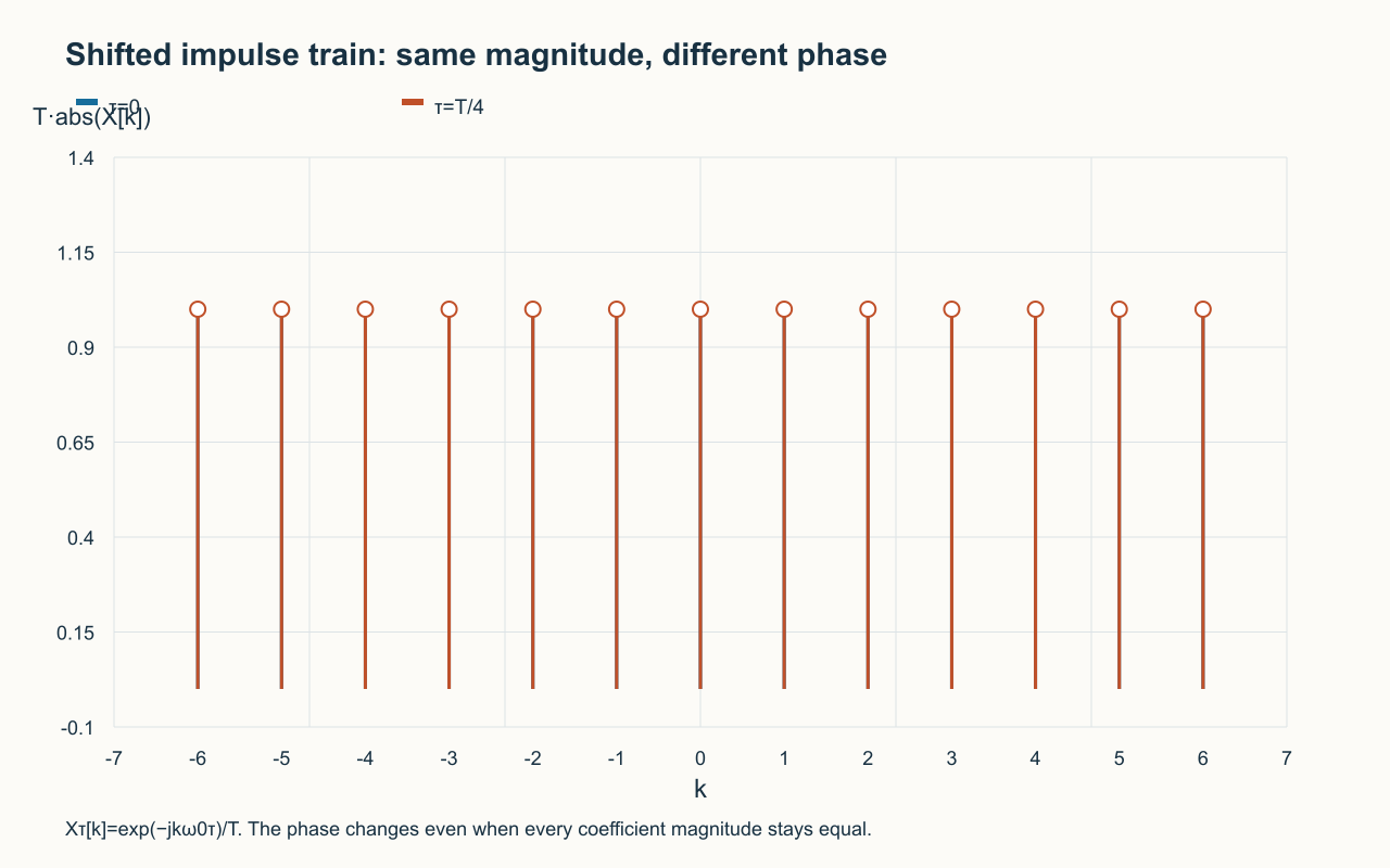
Shifting the impulse train by τ gives X[k]=exp(−jkω0τ)/T.Its magnitude is still 1/T, while its phase and time-domain location change. Flat magnitude alone does not identify a unique signal.Narration transcript
Let's visualize this remarkable result. Plotting the magnitude of X sub k versus k, we get a perfectly flat spectrum. Every harmonic from minus infinity to plus infinity has the exact same amplitude, one over T. This is why the impulse train is so fundamental in signal processing. It contains all frequencies with equal strength. No other periodic signal has this flat spectrum property.
5. Derivative method
Differentiate a piecewise smooth waveform distributionally; include an impulse with weight equal to every jump.Compute derivative coefficients and divide by jkω0 for k≠0; restore the mean separately.Narration transcript
Now let's put the differentiation property to practical use with what we call the derivative trick. When a signal has sharp transitions or discontinuities, computing Fourier coefficients directly can be very painful. Instead, we differentiate the signal. Discontinuities become impulses, and impulses have simple, known Fourier coefficients. We then recover the original coefficients by dividing: X sub k equals Y sub k divided by j k omega zero. This technique converts a difficult integration problem into simple algebra. Let's demonstrate on a square wave.
6. Square-wave coefficients
For period 2π and levels +m on (0,π), −m on (−π,0), the mean is zero.The derivative has a +2m jump impulse at zero and a −2m impulse at the other period boundary, counted once.F[k]=−j2m/(kπ) for odd k; coefficients are zero for nonzero even k, and F[0]=0.Narration transcript
Consider a square wave f of t with amplitude plus m for zero less than t less than pi, and minus m for negative pi less than t less than zero, with period T equals two pi. Computing F sub k directly requires careful integration. Instead, let's differentiate. The derivative g of t equals f prime of t produces impulse pairs at each discontinuity: positive two m times delta at t equals zero, and negative two m times delta at t equals plus or minus pi. Using our impulse result, G sub k equals m over pi times the quantity one minus cosine of k pi. Since cosine of k pi equals negative one to the k, for odd k this gives two m over pi, and for even k it gives zero. Dividing by j k to get F sub k, we obtain F sub k equals negative j times two m over k pi for odd k, and zero for even k.
7. Phasor interpretation
The paired positive and negative frequency components produce real sine terms with amplitudes 4m/(kπ) for positive odd k.Each individual complex coefficient has magnitude 2m/(abs(k)π); do not confuse it with the paired sine amplitude.Narration transcript
To develop intuition, let's visualize Fourier synthesis as rotating phasors. The fundamental harmonic k equals one traces a large circle in the complex plane, with radius four m over pi. The third harmonic k equals three traces a smaller circle, one third the radius, but rotating three times faster. The fifth harmonic is smaller still, one fifth the radius, five times the speed. As these phasors rotate, add their tips together. The sum traces out the time-domain signal. With just three harmonics, you can already see the square wave taking shape.
8. Partial sums
Add odd harmonics successively to approximate the square wave.At continuity points the series approaches the signal under the standard piecewise smooth conditions; at a jump it approaches the average of the one-sided limits.Narration transcript
Let's watch the convergence step by step. Starting with just the fundamental, f one of t equals four m over pi times sine t. It's a smooth sinusoid, the crudest possible approximation. Adding the third harmonic gives f two of t, with sine three t over three included. The waveform develops a hint of a flat top. With the fifth harmonic, f three of t shows clearer corners and flatter plateaus. By seven harmonics, the shape is unmistakably a square wave. But look carefully at the transitions. There are sharp oscillations that overshoot the target amplitude. These ripples don't disappear no matter how many terms we add.
9. Gibbs phenomenon
Near a jump, Fourier partial sums develop an overshoot tending to about 8.949% of the jump size.The affected region narrows as more terms are used, while the limiting peak overshoot does not vanish. At the jump itself the limit is the midpoint.Narration transcript
This persistent overshoot is the famous Gibbs phenomenon. At every discontinuity, the truncated Fourier series overshoots by approximately nine percent of the total jump. For our square wave with jump size two m, the overshoot is about zero point one eight m. As we add more harmonics, the overshoot gets narrower but its peak value stays at nine percent. The oscillations compress into a thinner region around the discontinuity, but the maximum overshoot never vanishes. This is not a failure of the Fourier series itself. The infinite series does converge correctly. It's specifically the truncation to finitely many terms that causes this effect.
10. Coefficient spectrum
Only odd harmonics remain, with complex magnitude 2m/(abs(k)π).The 1/abs(k) envelope reflects these jumps. Stronger smoothness, including matching periodic boundary derivatives, can yield faster decay.Narration transcript
Let's examine the coefficient spectrum of our square wave. Plotting the magnitude of F sub k versus k, we see a striking pattern. Only odd harmonics have nonzero coefficients, reflecting the half-wave symmetry. The magnitudes follow a one over k envelope, shown by the dashed curve. This slow one over k decay is characteristic of signals with jump discontinuities. Smoother signals would have spectra that decay much faster, like one over k squared or even exponentially.
11. Review
Corrected mathematical reference; use with the written derivation. State normalization, retain all derivative impulses and recover DC separately.An impulse train has flat magnitude, but phase prevents uniqueness. Distinguish paired sine amplitudes, complex coefficients and Gibbs behavior.Narration transcript
Let's review the five key results from today. First, scaling conventions: C1 times C2 must equal one over T in any Fourier pair. Second, differentiation in time multiplies coefficients by j k omega zero. Third, the periodic impulse train has a flat spectrum: X sub k equals one over T for all k. Fourth, the derivative trick turns discontinuities into impulses for easier coefficient computation. And fifth, truncated Fourier series exhibit the Gibbs phenomenon, a persistent nine percent overshoot at discontinuities. These tools are essential for analyzing any periodic signal in engineering.
Source video: Signals & Systems #23 | Fourier Series Properties - Square Wave, Derivative Trick & Gibbs (8:45)