Signals and Systems · Composite continuous-time signals

#10 Shifted impulses, steps, ramps and slope analysis

Build a rectangular pulse, a three-level staircase, a plateau and a triangle by tracking switching times and changes of slope.

Question

Original final-video graph or reference card for composite signals. — Original-video reference. Impulse labels denote weights. In the four-panel image the lower ramps are additional examples; the later worked plateau is height three. Plateau and triangle graphs are captured before the slope box covers the axis; their equations are developed in the notebook lines.

Use r(t)=max(t,0). For the plotted step endpoints choose u(0)=1: a shifted step turns on at its breakpoint. Impulse arrows carry unit weight, not an ordinary finite height. Solve each composite by activating its terms from left to right. At a ramp kink, report the slopes on the adjacent intervals; an ordinary derivative need not exist exactly at the kink. The general piecewise-linear construction also retains any initial affine baseline; impulses are separate singular components. The four-panel reference includes additional r(t−1) and 2r(t)−2r(t−3) examples. Keep that height-six plateau separate from the later height-three worked example. All worked examples here begin at zero before their first breakpoint.

Written solution and narration transcript(shows the full solution)

Below are all the lines written in the notebook together with the full narration transcript.

1. Choose elementary building blocks
Original-video reference. Impulse labels denote weights. In the four-panel image the lower ramps are additional examples; the later worked plateau is height three. Plateau and triangle graphs are captured before the slope box covers the axis; their equations are developed in the notebook lines.
Elementary blocks: δ(t), u(t), and r(t).
Write each composite as a sum of shifted and scaled building blocks.
Piecewise-linear construction: retain the initial affine baseline, then add steps for jumps and ramps for slope changes; impulses represent separate singular components.
Narration transcript
In the previous lectures, we learned three building blocks: the unit impulse delta of t, the unit step u of t, and the unit ramp r of t. Today we'll practice writing composite signals as combinations of these functions. The key idea is: any piecewise-linear signal can be built by adding shifted and scaled copies of delta, u, and r.
2. Locate two impulses and form a rectangular pulse
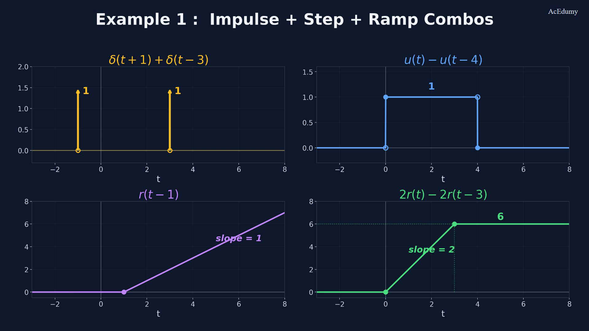
Original-video reference. Impulse labels denote weights. In the four-panel image the lower ramps are additional examples; the later worked plateau is height three. Plateau and triangle graphs are captured before the slope box covers the axis; their equations are developed in the notebook lines.
Begin with impulses and a step difference.
Two shifted impulses:
$\displaystyle g\left(t\right)=\delta \left(t+1\right)+\delta \left(t-3\right)$
Unit weights at negative one and three; arrow lengths are only a drawing convention.
Rectangular pulse:
$\displaystyle p\left(t\right)=u\left(t\right)-u\left(t-4\right)$
With the plotted right-continuous step convention, the pulse switches on at zero and off at four.
Unit height from zero (included) to four (excluded); zero elsewhere.
Narration transcript
Let's start with simple combinations. First, delta of t plus one plus delta of t minus three. This creates two impulse arrows: one at t equals negative one, and another at t equals three. Next, u of t minus u of t minus four. The first step turns on at t equals zero, and the second turns off at t equals four. The result is a rectangular pulse of width four and height one.
3. Add three shifted steps
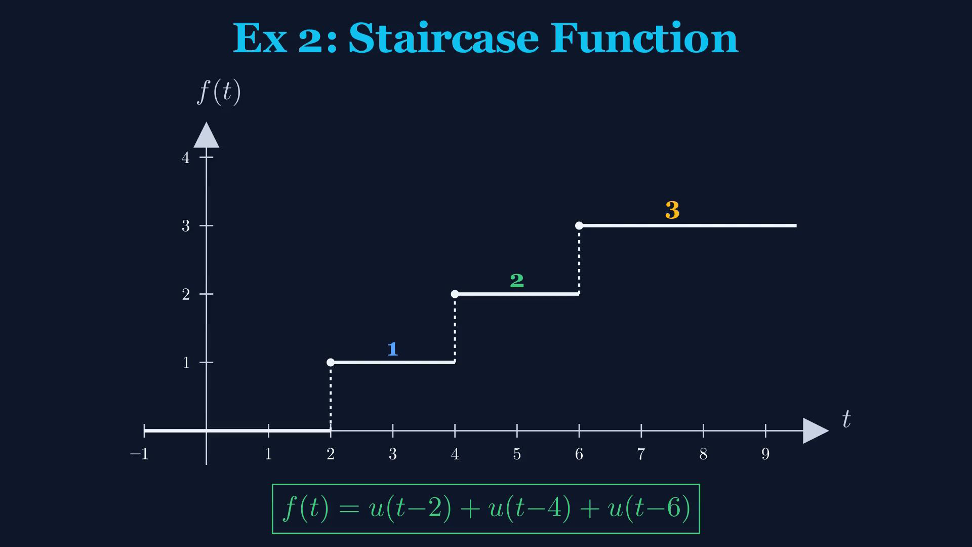
Original-video reference. Impulse labels denote weights. In the four-panel image the lower ramps are additional examples; the later worked plateau is height three. Plateau and triangle graphs are captured before the slope box covers the axis; their equations are developed in the notebook lines.
Three shifted steps:
$\displaystyle s\left(t\right)=u\left(t-2\right)+u\left(t-4\right)+u\left(t-6\right)$
Each new step adds one to the current level.
First level:
$\displaystyle s\left(2\right)=1+0+0=1$
Second level:
$\displaystyle s\left(4\right)=1+1+0=2$
Third level:
$\displaystyle s\left(6\right)=1+1+1=3$
Staircase levels: zero before two, then one, two and three.
Narration transcript
Now a staircase function: u of t minus two, plus u of t minus four, plus u of t minus six. Each shifted step adds one more level. At t equals two, the first step turns on, giving level one. At t equals four, the second step adds another one, reaching level two. At t equals six, the third step brings us to level three. The result is a perfect staircase.
4. Track slope changes between breakpoints
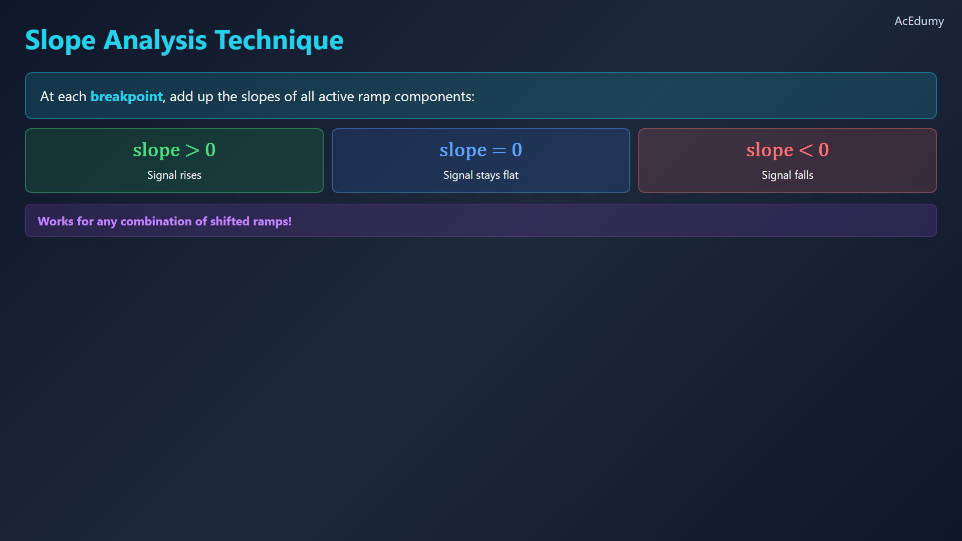
Original-video reference. Impulse labels denote weights. In the four-panel image the lower ramps are additional examples; the later worked plateau is height three. Plateau and triangle graphs are captured before the slope box covers the axis; their equations are developed in the notebook lines.
Slope analysis tracks the slopes contributed by active ramps.
At each breakpoint, update the slope on the next interval; the derivative at the kink may be undefined.
A positive slope makes the signal rise.
Zero slope makes the signal remain constant on that interval.
A negative slope makes the signal fall.
Add the active ramp slopes on every interval.
Narration transcript
For ramp combinations, we'll use a powerful technique called slope analysis. The idea is simple: at each breakpoint, add up the slopes of all active ramp components. If the total slope is plus one, the signal rises. If it drops to zero, the signal stays flat. If it goes negative, the signal falls. This method works for any combination of shifted ramps.
5. Cancel a ramp slope to reach a plateau
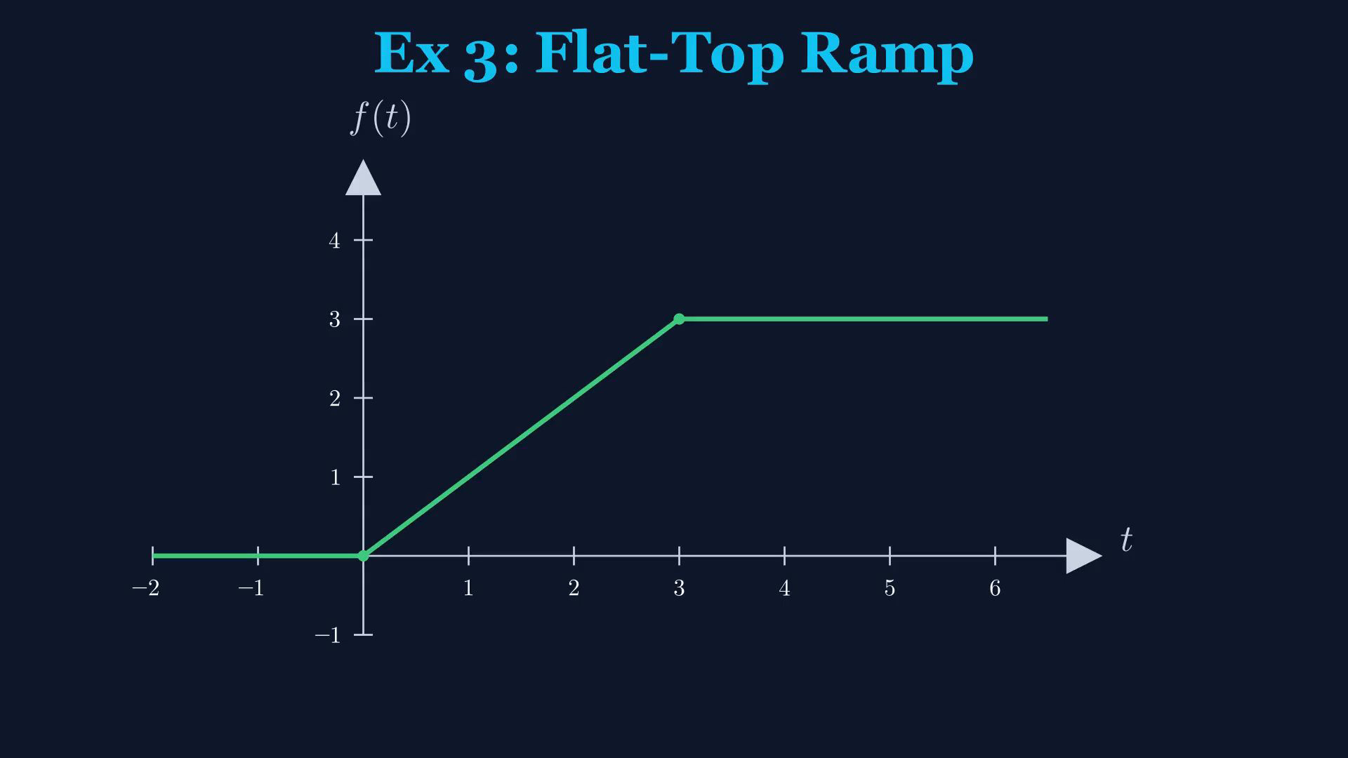
Original-video reference. Impulse labels denote weights. In the four-panel image the lower ramps are additional examples; the later worked plateau is height three. Plateau and triangle graphs are captured before the slope box covers the axis; their equations are developed in the notebook lines.
Plateau example:
$\displaystyle f\left(t\right)=r\left(t\right)-r\left(t-3\right)$
Before zero, both ramps vanish.
For 0<t<3:
$\displaystyle f\left(t\right)=t$
After three:
$\displaystyle f\left(t\right)=t-\left(t-3\right)=3$
Plateau height:
$\displaystyle f\left(3\right)=3-0=3$
The graph rises from zero to three and then remains at three.
Narration transcript
Let's apply slope analysis to r of t minus r of t minus three. Before t equals zero, nothing is active, so the slope is zero. At t equals zero, r of t turns on with slope plus one, so the signal rises linearly. At t equals three, the second ramp subtracts slope one, making the total slope zero. The signal levels off at a value of three. The result is a flat-top ramp: it rises from zero to three, then stays constant.
6. Build a triangle from three ramps
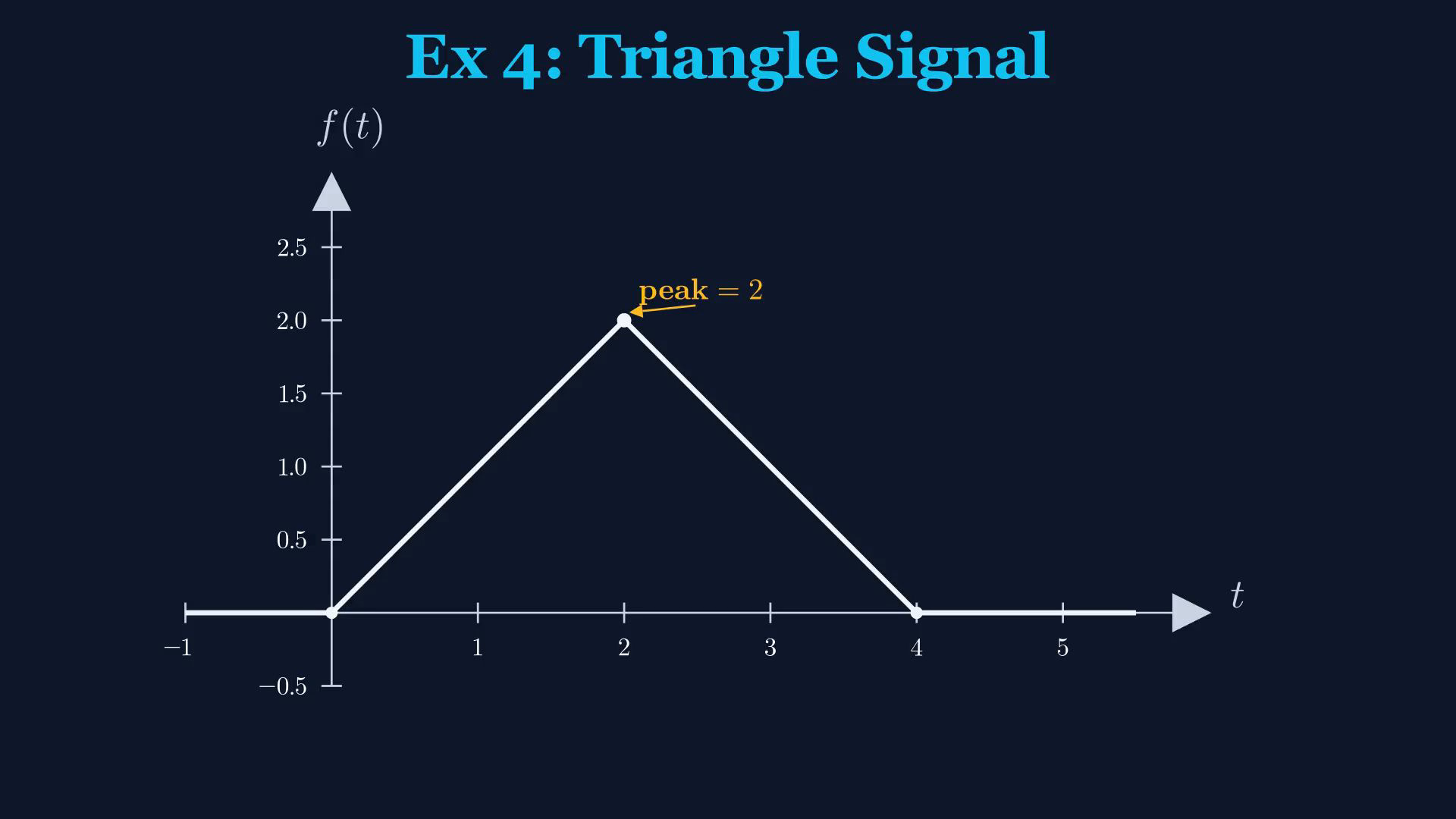
Original-video reference. Impulse labels denote weights. In the four-panel image the lower ramps are additional examples; the later worked plateau is height three. Plateau and triangle graphs are captured before the slope box covers the axis; their equations are developed in the notebook lines.
Triangle example:
$\displaystyle q\left(t\right)=r\left(t\right)-2r\left(t-2\right)+r\left(t-4\right)$
Before zero, all three terms vanish.
For 0<t<2:
$\displaystyle q\left(t\right)=t$
For 2<t<4:
$\displaystyle q\left(t\right)=t-2\left(t-2\right)=4-t$
The slope on this interval is negative one.
For t>4:
$\displaystyle q\left(t\right)=t-2\left(t-2\right)+\left(t-4\right)=0$
At the last breakpoint:
$\displaystyle q\left(4\right)=4-2\left(2\right)+0=0$
Triangle peak:
$\displaystyle q\left(2\right)=2$
Narration transcript
Our final example: r of t minus two r of t minus two plus r of t minus four. Before t equals zero, the slope is zero. At t equals zero, the first ramp starts with slope plus one. At t equals two, the second term subtracts slope two, making the net slope negative one. The signal starts decreasing. At t equals four, the third ramp adds slope plus one, making the net slope zero. But the value has already returned to zero. The result is a symmetric triangle: rising from zero to a peak of two at t equals two, then falling back to zero at t equals four.
7. Review jumps and slope changes
Original-video reference. Impulse labels denote weights. In the four-panel image the lower ramps are additional examples; the later worked plateau is height three. Plateau and triangle graphs are captured before the slope box covers the axis; their equations are developed in the notebook lines.
Composite signals combine elementary building blocks.
Impulse weights, step jumps and ramp slope changes play different roles.
List the slope on each interval and use continuity to carry values across ramp breakpoints.
Next: derivatives and impulses associated with jumps.
Narration transcript
To summarize: we practiced writing composite signals from building blocks. Shifted impulses create spikes, shifted steps create pulses and staircases, and shifted ramps create linear segments. The slope analysis technique is key for ramp combinations: list the slopes at each breakpoint, and the shape reveals itself. In the next lesson, we'll explore signal derivatives and how discontinuities produce impulses.