Signals and Systems · Continuous-time Fourier transform
#27 Periodic extension, transform samples and the inverse-transform limit
Derive the angular-frequency Fourier transform pair from a periodic extension and a Fourier-series Riemann sum.
Question
This derivation starts with an integrable finite-duration signal whose support lies strictly inside a centered interval of length T. Choose T large enough that periodic copies do not overlap. Define p(t) as the periodic extension called x-tilde in the narration and C[k] as its Fourier-series coefficients called capital X-tilde; X(omega) is the continuous-frequency Fourier transform of the original x(t), and these are different objects. Periodic p equals x only within that chosen central period, not on the entire real line. The original x is zero outside its support, allowing its coefficient integral to extend to both infinities. For signals with infinite support the nonoverlap argument is not literal; periodization needs separate convergence justification. Omega is angular frequency in radians per unit time, with omega0 equal to two pi divided by T and k an integer. The direct Fourier transform uses a negative exponential and no prefactor; the inverse uses a positive exponential and one divided by two pi. The sampling relation C[k]=X(k omega0)/T holds for the stated periodization and standard transform convention. In the limit, the frequency grid becomes dense as omega0 tends to zero; it is not the claim that a fixed k reaches arbitrary omega. The sum includes its frequency-width factor omega0, and the Riemann-sum limit needs convergence justification. The introductory phrase about any aperiodic signal is a broad preview, not an existence theorem: aperiodicity alone does not ensure a convergent ordinary Fourier integral. Use the finite-duration assumptions here and the convergence conditions introduced next. For example, absolute integrability ensures the ordinary forward transform; appropriate inverse conditions give equality at continuous points and midpoint values at jumps for piecewise smooth signals. Square-integrable and distributional Fourier transforms require their own meanings and are not ordinary integrals by default. Never claim arbitrary functions have these integrals. In the general convention, c1 and c2 are nonzero constants whose product is one divided by two pi; changing c1 rescales X, so standard and symmetric spectra are not numerically identical. Both constants equal one divided by the square root of the complete quantity two pi in the symmetric convention. The signal sketches are schematic with separate axes, not measurements of identical pixel widths.
Written solution and narration transcript(shows the full solution)
Below are all the lines written in the notebook together with the full narration transcript.
1. From periodic to aperiodic
Original-video reference. In the written steps, p(t) is the periodic extension labeled x-tilde in the video, and C[k] are its Fourier-series coefficients labeled capital X-tilde. The finite-duration signal fits inside one period without overlap. The inverse integral is interpreted with the appropriate convergence conditions, discussed in the following lesson; aperiodicity alone does not guarantee ordinary integral convergence. The small pulse sketches are schematic and use separate horizontal scales. Recall Fourier series for periodic signals.Consider signals that do not repeat periodically.Examples include a single pulse and a decaying exponential.A Fourier series represents periodic repetition.Extend frequency analysis to aperiodic signals.Derive the transform by increasing the repetition period without bound.Introduce the FT and inverse FT pair; their convergence conditions still apply.Narration transcript
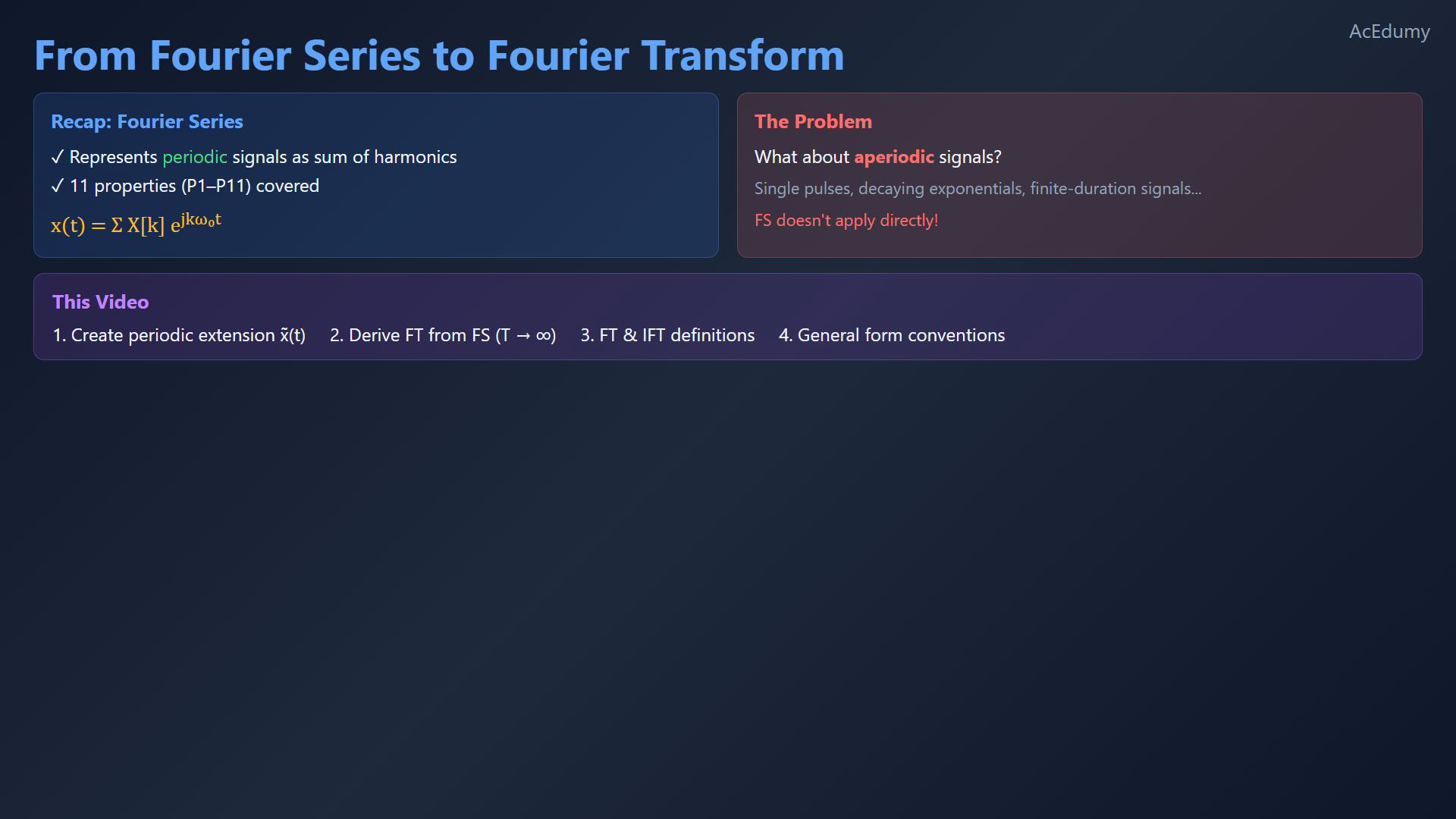
In the previous videos, we explored Fourier Series and its eleven properties for periodic signals. But here's a natural question: what about signals that are NOT periodic? Aperiodic signals, like a single rectangular pulse or a decaying exponential, don't repeat forever. So we can't directly apply Fourier Series to them. In this video, we'll bridge that gap. We'll derive the Continuous-Time Fourier Transform by starting from Fourier Series and taking the period to infinity. By the end, you'll have the FT and Inverse FT formulas that work for any aperiodic signal.
2. Repeat a finite-duration signal
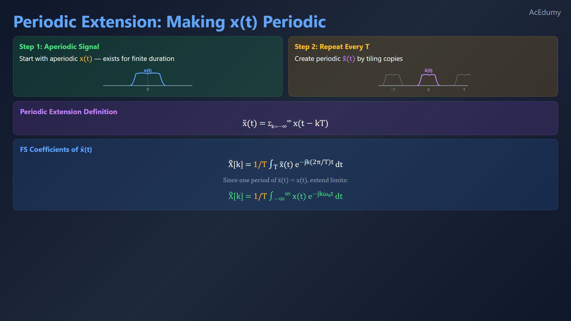
Original-video reference. In the written steps, p(t) is the periodic extension labeled x-tilde in the video, and C[k] are its Fourier-series coefficients labeled capital X-tilde. The finite-duration signal fits inside one period without overlap. The inverse integral is interpreted with the appropriate convergence conditions, discussed in the following lesson; aperiodicity alone does not guarantee ordinary integral convergence. The small pulse sketches are schematic and use separate horizontal scales. Begin with a finite-duration signal.Choose a full period containing its support.Repeat the signal every T seconds without overlap.Write the periodic extension as p:This tiles copies along the time axis.Inside the selected central period, the periodic extension equals the original.Apply Fourier series to the periodic extension.Write its coefficients as C:Now use the finite support of the original signal.Since the original vanishes outside this interval, extend its integral limits.The original-signal integral is:Narration transcript
Here's the key idea. Suppose we have an aperiodic signal x of t, maybe a pulse that exists only for a finite duration. We can artificially make it periodic by repeating copies every T seconds. This creates a periodic signal x-tilde of t, defined as the sum from k equals negative infinity to positive infinity of x of t minus k T. Think of it as tiling x of t along the time axis. One period of x-tilde is exactly our original x of t. Since x-tilde is periodic with period T, we CAN apply Fourier Series to it. The FS coefficients are: x-tilde of k equals one over T times the integral over one period of x-tilde of t times e to the minus j k two pi over T t, dt. Now here's the crucial step. Since one period of x-tilde is just x of t, and x of t is zero outside that interval, we can extend the integration limits to negative infinity to positive infinity. So x-tilde of k equals one over T times the integral from negative infinity to positive infinity of x of t, e to the minus j k omega-zero t, dt.
3. Define the Fourier transform
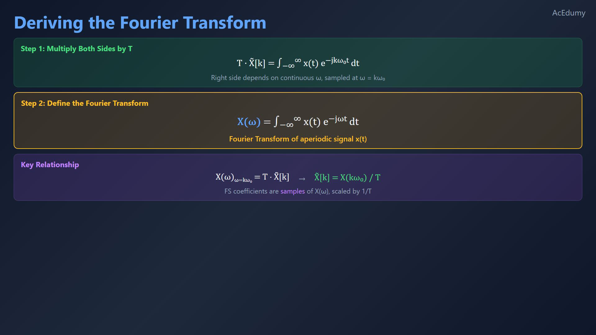
Original-video reference. In the written steps, p(t) is the periodic extension labeled x-tilde in the video, and C[k] are its Fourier-series coefficients labeled capital X-tilde. The finite-duration signal fits inside one period without overlap. The inverse integral is interpreted with the appropriate convergence conditions, discussed in the following lesson; aperiodicity alone does not guarantee ordinary integral convergence. The small pulse sketches are schematic and use separate horizontal scales. Read a continuous-frequency function from the coefficient integral.Multiply both sides by the period.The scaled coefficients are:Sample at harmonic angular frequencies:Define the standard forward transform:This transforms the original aperiodic signal under the stated conditions.The transform samples and periodic coefficients satisfy:Divide each transform sample by the period:Narration transcript
Now let's extract something powerful from this expression. Multiply both sides by T. We get: T times x-tilde of k equals the integral from negative infinity to infinity of x of t, e to the minus j k omega-zero t, dt. The right side depends on the continuous variable omega, evaluated at discrete points omega equals k omega-zero. So we define a new function: X of omega equals the integral from negative infinity to infinity of x of t, e to the minus j omega t, dt. This is the Fourier Transform of the aperiodic signal x of t. Notice the key relationship: X of omega, evaluated at omega equals k omega-zero, gives us T times the FS coefficients of the periodic extension. In other words, the FS coefficients are samples of X of omega, divided by T: x-tilde of k equals X of k omega-zero, divided by T.
4. Take the inverse-transform limit
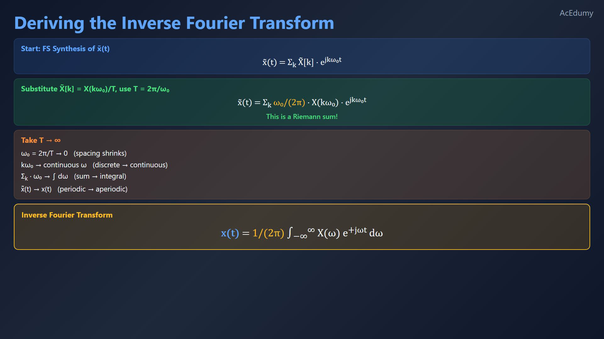
Original-video reference. In the written steps, p(t) is the periodic extension labeled x-tilde in the video, and C[k] are its Fourier-series coefficients labeled capital X-tilde. The finite-duration signal fits inside one period without overlap. The inverse integral is interpreted with the appropriate convergence conditions, discussed in the following lesson; aperiodicity alone does not guarantee ordinary integral convergence. The small pulse sketches are schematic and use separate horizontal scales. Derive the inverse transform.Start with periodic synthesis:Substitute the sampled transform and frequency width:Inspect the frequency-width factor in this sum.It has the form of a Riemann sum.As the period grows, the frequency spacing tends to zero:The grid becomes dense and the weighted sum tends to an integral when justified.The standard inverse formula is:This is the inverse Fourier transform, with the appropriate convergence interpretation.Narration transcript
Now let's derive the inverse transform. The Fourier Series synthesis equation for x-tilde is: x-tilde of t equals the sum over k of x-tilde of k, times e to the j k omega-zero t. Substituting x-tilde of k equals X of k omega-zero over T, and using T equals two pi over omega-zero, we get: x-tilde of t equals the sum over k of omega-zero over two pi, times X of k omega-zero, times e to the j k omega-zero t. Look carefully. This is a Riemann sum! As T goes to infinity, omega-zero, which equals two pi over T, approaches zero. The discrete frequencies k omega-zero become the continuous variable omega, and the sum becomes an integral. In the limit, x-tilde of t approaches x of t, and we obtain: x of t equals one over two pi, times the integral from negative infinity to infinity of X of omega, e to the j omega t, d-omega. This is the Inverse Fourier Transform.
5. Transform conventions
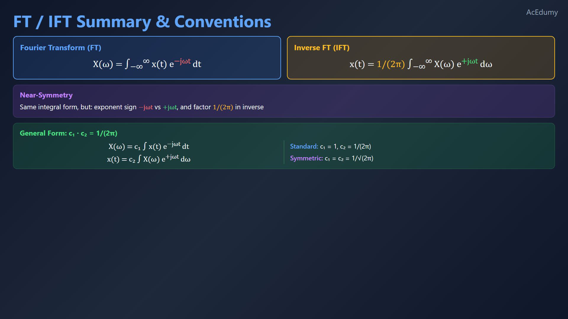
Original-video reference. In the written steps, p(t) is the periodic extension labeled x-tilde in the video, and C[k] are its Fourier-series coefficients labeled capital X-tilde. The finite-duration signal fits inside one period without overlap. The inverse integral is interpreted with the appropriate convergence conditions, discussed in the following lesson; aperiodicity alone does not guarantee ordinary integral convergence. The small pulse sketches are schematic and use separate horizontal scales. Collect the transform pair.Forward transform under the stated conditions:Inverse transform under the stated conditions:Observe the near symmetry of the two integrals.Their exponent signs are opposite; the inverse has one divided by two pi.For general angular-frequency conventions:The standard convention is:The symmetric convention is:The transform extends frequency analysis to aperiodic signals with suitable interpretations.Next: convergence conditions and the first transform examples.Narration transcript
Let's put it all together. For an aperiodic signal x of t, the Fourier Transform pair is: Forward transform: X of omega equals the integral from minus infinity to infinity of x of t, e to the minus j omega t, dt. Inverse transform: x of t equals one over two pi, times the integral from minus infinity to infinity of X of omega, e to the plus j omega t, d-omega. Notice the beautiful near-symmetry. Both are integrals of the same form, but with opposite exponent signs and a factor of one over two pi in the inverse. In general, we can define the pair with constants c-one and c-two, where c-one times c-two must equal one over two pi. Our convention uses c-one equals 1 and c-two equals one over two pi. Another popular choice is the symmetric form, where both constants equal one over the square root of two pi. Regardless of convention, the Fourier Transform extends frequency analysis from periodic signals to aperiodic signals. In the next video, we'll discuss convergence conditions and compute our first Fourier Transform examples.
Source video: Signals & Systems #27 | CT Fourier Transform - From FS to FT (5:55)